Structural Geology - Data Preparation
< Previous section Next section >
For our analyses, the data must be prepared carefully to ensure that all required information is available. In particular, we need a mapping between each point and its corresponding scanner position. This mapping is later used for correct surface normal orientation, as it allows us to determine whether a normal vector points into the rock mass (for example on vertical or overhanging sections) and therefore needs to be flipped to point outward.
The scanner position layer contains two attributes: an identifier (Id) for the scan position (1–3) and the elevation (Z).
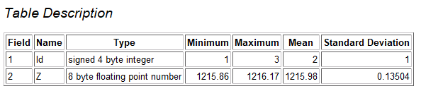
The attributes of the scanner position point layer.
The point clouds themselves only contain the scan position identifier in their filenames. We therefore use the “Add Input Identifier” option of the “Merge Point Clouds” tool to assign a unique identifier to each point while merging the three scans into a single point cloud dataset. The identifier value is incremented automatically for each input point cloud starting from the specified initial value, which means that the order of the input point clouds is important. Add them exactly in this order: scan_1, scan_2, scan_3.
Enable the “Add Input Identifier” option. The “Delete Input” option removes the three input point clouds after merging in order to free memory resources.
Tool: Merge Point Clouds
Geoprocessing → Shapes → Point Clouds → Tools // Tools → Shapes → Point Clouds
| Parameter | Setting |
|---|---|
| Data Objects | |
| Point Clouds | |
| >> Point Clouds | 3 objects (scan_1, scan_2, scan_3) |
| << Merged Point Cloud | <create> |
| Options | |
| Delete Input | 🗹 |
| Add Input Identifier | 🗹 |
| Start Value | 1 |
We now have a single point cloud dataset containing a new attribute that maps each point to its corresponding scanner position (1–3).
Because the dataset combines scans acquired from three different positions, the point density varies throughout the point cloud. In areas where scans overlap, the data is oversampled. To achieve a spatially uniform point density and ensure consistent results in subsequent analyses, we therefore perform a data homogenization step.
For this purpose, we apply a 3D block thinning operation that retains the point closest to the center of each voxel. For this tutorial, and to keep the dataset size manageable, we use a voxel size of 3 × 3 × 3 cm.
Tool: Block Thinning 3D
Geoprocessing → LIS Pro 3D → Thinning → Point Cloud // Tools → LIS Pro 3D → Thinning
| Parameter | Setting |
|---|---|
| Data Objects | |
| Point Clouds | |
| >> Point Cloud | Merged |
| Filter Attribute | <not set> |
| << Point Cloud Thinned | <create> |
| Options | |
| Copy existing Attributes | 🗹 |
| Method Thinning | nearest |
| Horizontal Spacing | 0.03 |
| Vertical Spacing | 0.03 |
| Point Count Filter | ☐ |
| Method Baseline | lowest point |
A more sophisticated thinning strategy could be based on the laser beam incidence angle, since high incidence angles generally result in larger positional errors. The incidence angle can be computed using the “Point Cloud Accuracy Estimation” tool. The 3D block thinning could then be performed using the “min(attribute)” method, retaining the point with the lowest incidence angle and therefore the highest positional accuracy within each voxel.
Please rename the output point cloud (“Merged_thinned”) to “rock_face” or another meaningful name. You can now close the unthinned point cloud dataset to free memory resources if desired. Save the “rock_face” point cloud to disk.
As a final preprocessing step, we establish the mapping between each point and its corresponding scanner position and create a “direction-to-scanner” attribute for every point. This attribute stores a unit vector pointing from each point toward the scanner position from which it was acquired.
Because this is a three-dimensional vector, three separate attributes are created, one for each vector component (x, y, and z). These attributes will later be used to orient surface normal vectors correctly.
Open the “Map Point Cloud to Scanner” tool. For the “Method” parameter, select “Point Source ID”. This option allows you to use the scan position identifier attributes for establishing the mapping.
Tool: Map Point Cloud to Scanner
Geoprocessing → LIS Pro 3D → Tools → Point Cloud // Tools → LIS Pro 3D → Tools
| Parameter | Setting |
|---|---|
| Data Objects | |
| Point Clouds | |
| >> Point Cloud | rock_face |
| Point Source ID | ID |
| < Point Cloud | <not set> |
| Shapes | |
| >> Scanner Position(s) | scan_positions |
| Point Source ID | Id |
| Z | Z |
| Options | |
| Copy existing attributes | 🗹 |
| Attribute Suffix | |
| Method | point source id |
| Direction to Scanner | 🗹 |
| Position of Scanner | ☐ |
| Range to Scanner | ☐ |
| Polar Angle | ☐ |
| Azimuthal Angle | ☐ |
The point cloud dataset is now ready for the subsequent analysis steps. Please save the data again.
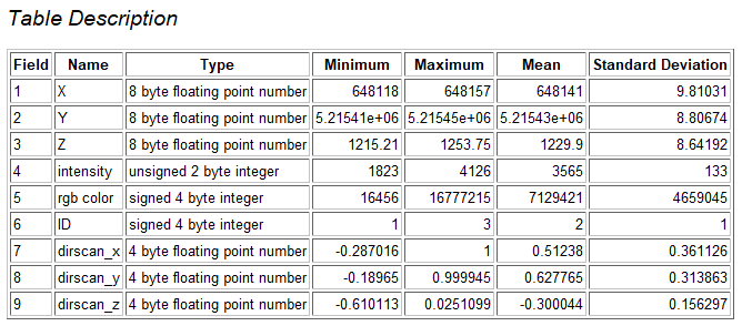
The attributes of the preprocessed point cloud.
Finally, we can inspect the point cloud in 3D using the Point Cloud Editor tool. Provide the intensity, RGB color, and ID attribute fields to enable switching between different colorizations using the keyboard shortcuts.
Tool: Point Cloud Editor
Geoprocessing → LIS Pro 3D → Point Cloud Editor // Tools → LIS Pro 3D → Point Cloud Editor
| Parameter | Setting |
|---|---|
| Data Objects | |
| Point Clouds | |
| >> Point Cloud | rock_face |
| Intensity | intensity |
| RGB | rgb color |
| Shading | <not set> |
| Classification | <not set> |
| Random | ID |
| Normal Vector (X) | <not set> |
| Report Attribute 1 | <not set> |
| Report Attribute 2 | <not set> |
| Grids | |
| > Elevation Grids | No objects |
| > Color Grids | No objects |
| Shapes | |
| > Shapes | <not set> |
| Options | |
| Work on Copy of Point Cloud | ☐ |
| Background Color | #3C3C32 |
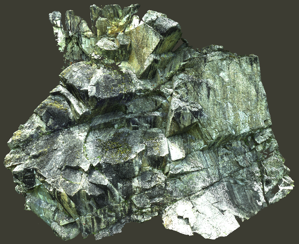 The point cloud visualized in true color (keyboard shortcut “3”).
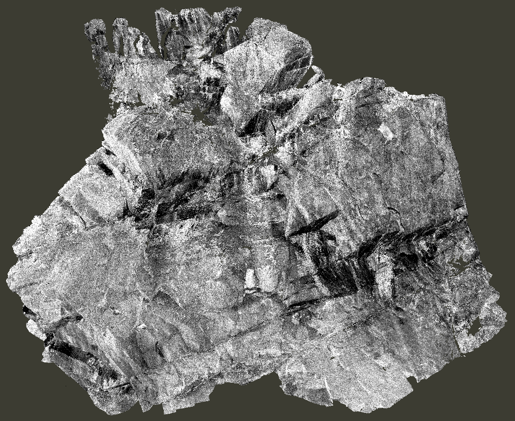 The point cloud visualized using intensity values (keyboard shortcut “2”).
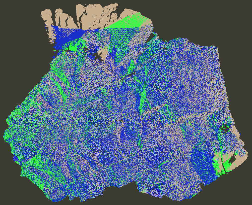 The point cloud colored by scan position (random colors, keyboard shortcut “q”). This view allows us to distinguish points originating from the three different scan positions.