Downloading & Preparing Data
Overview
In this tutorial, you will learn how you can combine digital terrain models, point clouds and building footprings to derive true LOD2 (level-of-detail 2) building models. Along the way, real, planar roof segments will be derived directly from from the point cloud data. Finally, the output will be saved in the widely used formats CityGML and CityJSON formats. This allows their usage in specialized downstream software (e.g., a webviewer).
Such LOD2 building models are the basis for modelling the solar potential for vertical building walls and individual roof segments. Other applications are the integration in digital twins and their usage for urban modelling studies (e.g., to simulate fine-scale meteorology, inundation mapping, noise modelling)
Downloading Tutorial Data
Here you can download a number of laz-files and shapefiles, which we will use throughout this tutorial. This data is available from the Canton of Zurich under the CC-BY-4.0 license.
Download the entire CityModeller directory. This should include the following files:
├── lidar
|   ├── DTMs
|   |   ├── 2684000_1246000.tif
|   |   ├── 2684000_1246500.tif
|   |   ├── 2684500_1246000.tif
|   |   └── 2684500_1246500.tif
|   └── pointclouds
|       ├── 2684000_1246000.laz
|       ├── 2684000_1246500.laz
|       ├── 2684500_1246000.laz
|       └── 2684500_1246500.laz
├── vector
|   └── Amtliche_Vermessung_-_Datenmodell_ZH_-Standard-_-OGD
|       ├── Bo_BoFlaeche_A.shp
|       └── ...
├── DATASOURCE
└── LICENSE
Open Vector Layer in LIS Pro 3D
Open LIS Pro 3D (e.g. by using the desktop shortcut)

In the upper-left corner of the LIS Pro 3D GUI, select File > Data > Shapes
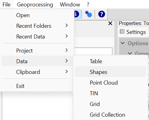
Navigate to your vector folder and select the shapefile Bo_BoFlaeche_A.shp
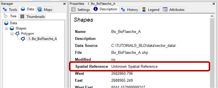
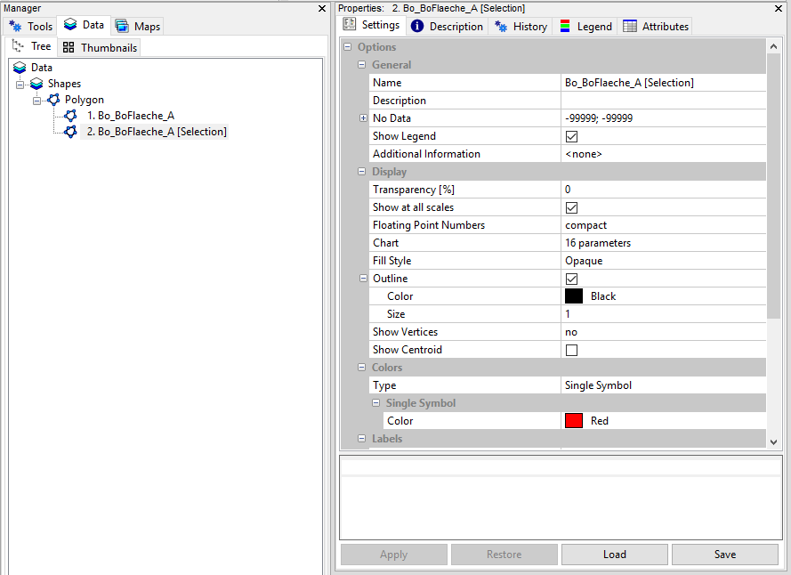
In LIS Pro 3D select the Data Tab in the Manager Window and the Description Tab in the Properties Window.
You can see that the layer was loaded, but it still has no spatial reference assigned.
Set Spatial Reference for Layer
Go to the Tools Tab of the Manager Window and set the coordinat system with the following tool:
In all our tutorials, we describe the execution of individual tools via the Tool Libraries interface. If you are not familiar with executing tools this way, please consult this section in our introductory tutorial series. In this section, we describe how you can locate the tools in LIS Pro 3D’s GUI.
Tool: Set Coordinate Reference System
Geoprocessing → Projection → Tools // Tools → Projection → PROJ
| Parameter | Setting |
|---|---|
| Options | |
| Definition String | +proj=somerc +lat_0=46.95240555555556 +lon_0=7.439583333333333 +k_0=1 +x_0=2600000 +y_0=1200000 +ellps=bessel +towgs84=674.374,15.056,405.346,0,0,0,0 +units=m +no_defs |
| Display Definition as… | PROJ |
| Authority Code | 2056 |
| Authority | EPSG |
| Geographic Coordinate Systems | <select> |
| Projected Coordinate Systems | <select> |
| Well Known Text File | |
| Pick from Data Set | 3 parameters |
| Customize | 165 parameters |
| Data Objects | |
| Grids | |
| > Grids | No objects |
| Shapes | |
| > Shapes | 1 object (Bo_BoFlaeche_A) |
- In the Authority Code section fill in the EPSG Code 2056 (The Projected Coordinate System for Switzerland CH1903+ / LV95).
- In the Shapes Section, provide the shapefile we have just loaded.
- Click Execute
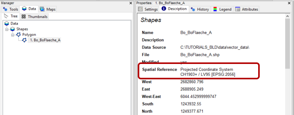
After this, we select the Data Tab in the Manager Window again.
In the Description Tab of the Properties Window we can see that the spatial reference is now assigned.
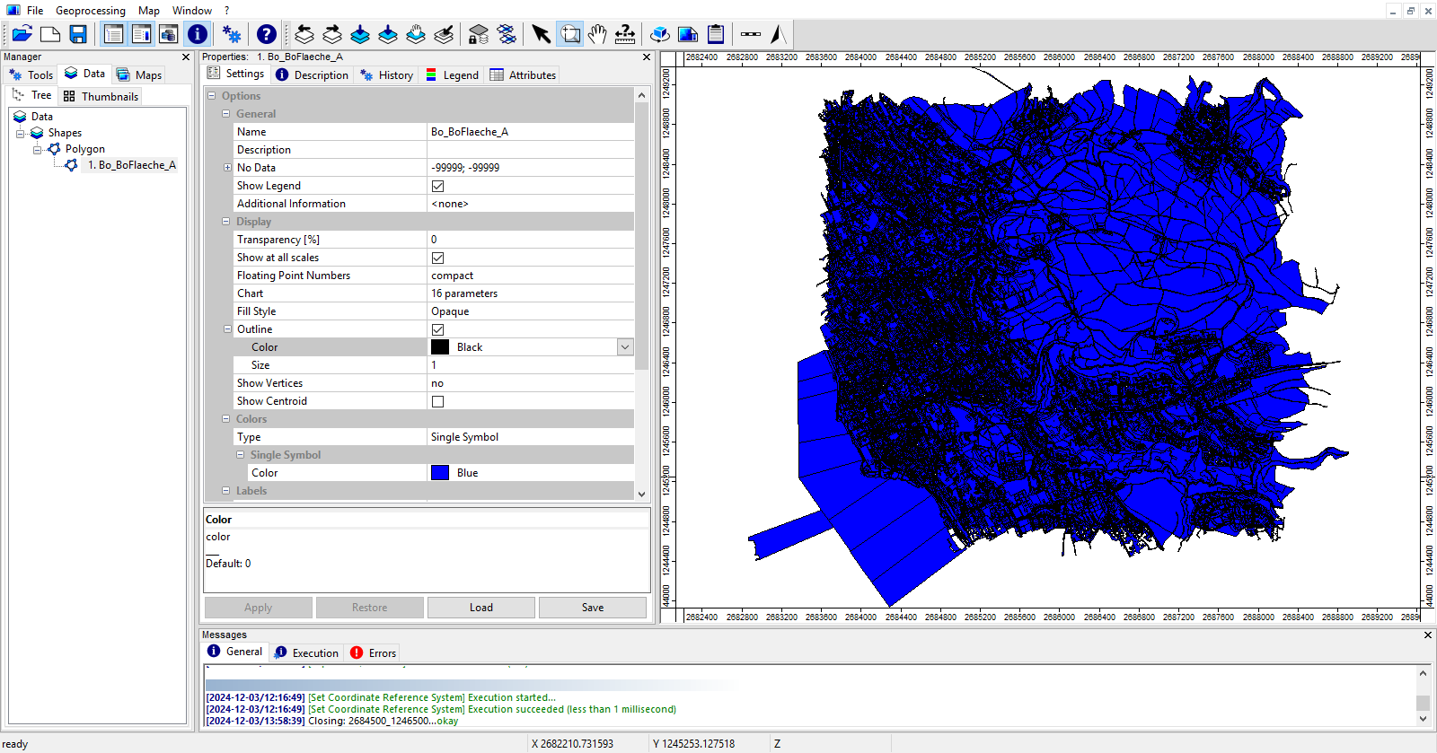
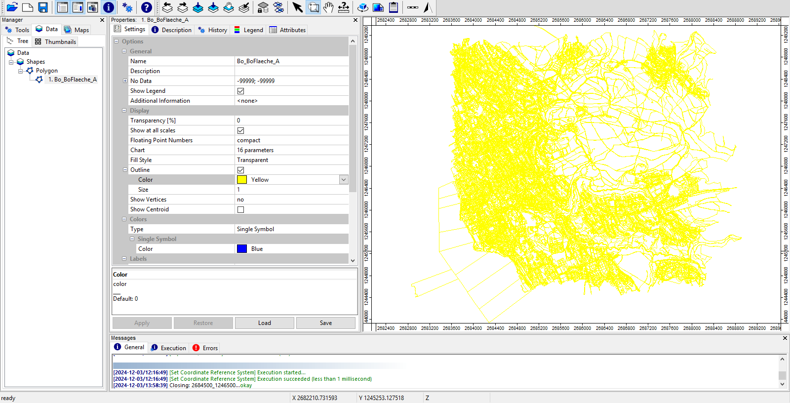
View the Layer in a Map View
Double-click onto the Bo_BoFlaeche_A Layer in the Data Tab.
This will show the layer in a map.
Change View Type of Layer
With the Data Tab selected and the Settings Tab of the Properties Window selected,
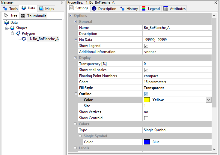
- Set the Fill Style to transparent
- Set the (Outline) Color to Yellow
- Click Apply
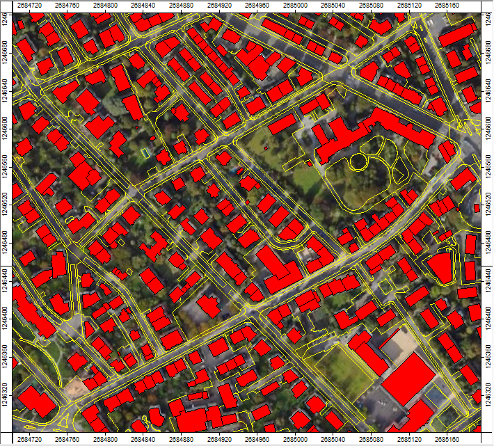
Add a WMS Base Layer
In the top menu, select Map > Add Base Map
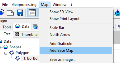
Choose Google Satellite and click Okay.
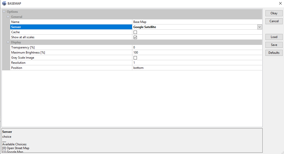
This will load a Base Map into your Map.
Use the Zoom Tool and drag a rectangle in the map, in order to zoom in.
alternatively use the mouse wheel for zooming in and out
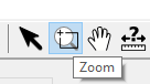
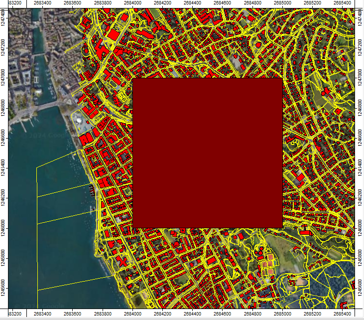
We can see, that the Base Map and the Vector Layer are quite well aligned.
Select and Copy Building Shapes from Layer
The shapefile has the attributes ART and ART_TXT with the following meaning:
| ART | ART_TXT |
|---|---|
| 0 | Gebaeude.Verwaltung |
| 1 | Gebaeude.Wohngebaeude |
| 2 | Gebaeude.Land_Forstwirtschaft_Gaertnerei |
| 3 | Gebaeude.Verkehr |
| 4 | Gebaeude.Handel |
| 5 | Gebaeude.Industrie_Gewerbe |
| 6 | Gebaeude.Gastgewerbe |
| 7 | Gebaeude.Nebengebaeude |
| 8 | befestigt.Strasse_Weg.Strasse |
| … | … |
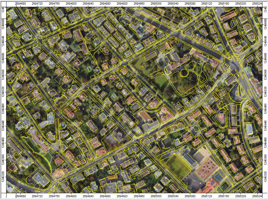
ART 0-7 are different types of buildings (Gebäude)
Now select and copy all the different types of buildings in the layer:
Tool: Select by Attributes… (Numerical Expression)
Geoprocessing → Shapes → Selection // Tools → Shapes → Tools
| Parameter | Setting |
|---|---|
| Data Objects | |
| Shapes | |
| >> Shapes | Bo_BoFlaeche_A |
| Attribute | ART |
| << Copy | <create> |
| Options | |
| Expression | a < 8 |
| Inverse | ☐ |
| Use No-Data | ☐ |
| Method | new selection |
| Post Job | copy |
- Provide the building layer Bo_BoFlaeche_A
- Provide the Attribute ART.
- Define an Expression: a < 8
- Click Execute
This will select and copy the buildings only
In the Data Tab a new polygon layer appears.
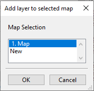
Double-click onto the new layer and add it to the existing map (Don’t select New).
A building layer is now visible in the map.
Rename the New Layer
Select the new polygon layer in the Data Tab and the Settings Tab in the Properties Window
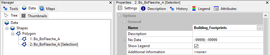
- Provide a new Name: Building_Footprints
- Click Apply
Add Unique Identifier to Buildings
In order to ensure that each building has a unique identifier, we create an additional attribute field for the given shapefile:
Tool: Field Enumeration
Geoprocessing → Table → Tools;Shapes → Attributes // Tools → Table → Tools
| Parameter | Setting |
|---|---|
| Data Objects | |
| Tables | |
| >> Input | Building_Footprints |
| Attribute | <not set> |
| Enumeration | <not set> |
| Shapes | |
| < Result | <not set> |
| Options | |
| Enumeration Field Name | proc_id |
| Order | ascending |
- Provide the shapefile
- Change the field name to proc_id
- Click Execute
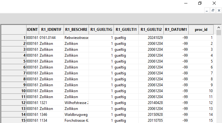
Right-click onto the shapefile in the Data Tab and choose Attributes > Show Table.
This will show the Attributes Table of the shapesfile (including the ART and ART_TXT attributes). We can see that the last attribute is the one that we have just created (proc_id):
Save the Building Dataset to Disk
Right-click onto the Building_Footprint layer in the Data Tab and select Save as
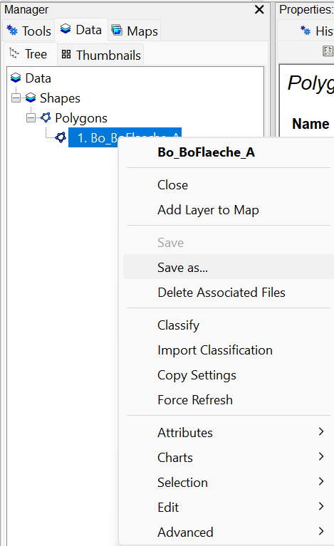
Save it to the vector folder.
Prepare LiDAR Data
Create Catalog of Raster Files
You have 4 raster files available in the DTMs folder. Now we want to create a catalog that allows seamless access to them via a virtual raster:
Tool: Create Virtual Raster (VRT) Geoprocessing → File → Grid // Tools → Import/Export → GDAL/OGR
| Parameter | Setting |
|---|---|
| Options | |
| Files | “C:\\..\lidar\DTMs\2684000_1246000.tif” “C:\\..\lidar\DTMs\2684000_1246500.tif” “C:\\..\lidar\DTMs\2684500_1246000.tif” “C:\\..\lidar\DTMs\2684500_1246500.tif” |
| VRT Filename | C:\\…\lidar\DTMs\tiles.vrt |
| Resampling | nearest |
| Resolution | highest |
- Use the browse button in the Files section to select the 4 downloaded tif-files in the DTMs folder
- Use the browse button in the VRT Filename section to define the output file called tiles.vrt in the very same DTMs folder
- Click Execute
Create Shape Layer for Raster Catalog
As we have now created a raster catalog for our 4 input DTMs, we can try to get a quick overview for the extent of the four datasets. Therefore we will create a shape layer that contains a polygon for each of the underlying raster files:
Tool: Create Raster Catalogue from Virtual Raster (VRT)
Geoprocessing → File → Grid // Tools → Import/Export → GDAL/OGR
| Parameter | Setting |
|---|---|
| Options | |
| VRT File | C:\\…\lidar\DTMs\tiles.vrt |
| Data Objects | |
| Shapes | |
| << Raster Catalogue | <create> |
- Select the previously created VRT file in the DTMs folder
- Click Execute
- A new polygon shapefile will appear in the Data Tab
Set Projection for Tileshape
Now set the correct coordinate system for the shape layer tileshape that defines the processing units:
Tool: Set Coordinate Reference System
Geoprocessing → Projection → Tools // Tools → Projection → PROJ
| Parameter | Setting |
|---|---|
| Options | |
| Definition String | +proj=somerc +lat_0=46.95240555555556 +lon_0=7.439583333333333 +k_0=1 +x_0=2600000 +y_0=1200000 +ellps=bessel +towgs84=674.374,15.056,405.346,0,0,0,0 +units=m +no_defs |
| Display Definition as… | PROJ |
| Authority Code | 2056 |
| Authority | EPSG |
| Geographic Coordinate Systems | <select> |
| Projected Coordinate Systems | <select> |
| Well Known Text File | |
| Pick from Data Set | 3 parameters |
| Customize | 165 parameters |
| Data Objects | |
| Grids | |
| > Grid | No objects |
| Shapes | |
| > Shapes | 1 object (Raster Catalogue) |
- In the Authority Code section fill in the EPSG Code 2056 (The Projected Coordinate System for Switzerland CH1903+ / LV95).
- In the Shapes Section, provide the tileshape we have just created
- Click Execute
Add Raster Catalog to Map
Double click the Raster Catalog in order to add it to the map:
Create Point Cloud Catalog
Now we would like to create a catalog for the pointclouds to enable seamless access:
Create Index-File for Efficient Access
First, we will create a las/laz-index for efficient data access:
Tool: Create LAS/LAZ Index
Geoprocessing → LIS Pro 3D → Import/Export → LAS/LAZ // Tools → LIS Pro 3D → Import/Export
| Parameter | Setting |
|---|---|
| Options | |
| Input Files | “C:\\…\lidar\pointclouds\2684000_1246000.laz” “C:\\…\lidar\pointclouds\2684000_1246500.laz” “C:\\…\lidar\pointclouds\2684500_1246000.laz” “C:\\…\lidar\pointclouds\2684500_1246500.laz” |
| Input File List | |
| Index All Files | 🗹 |
| Indexing | |
| Tile Size | 0 |
| Threshold | 1000 |
| Adaptive Coarsening | |
| Minimum Point Count | 100000 |
| Maximum Interval Count | -20 |
- In the Input Files section, select all available laz files in the pointclouds folder
- Click Execute
This will create lax-files in the same folder as your laz-files. These files will not show up directly in SAGA GIS & LIS Pro 3D, they will only be accessed by tools later in the background!
Create the Point Cloud Catalog
Tool: Create Virtual LAS/LAZ Dataset
Geoprocessing → LIS Pro 3D → Virtual → LAS/LAZ // Tools → LIS Pro 3D → Virtual
| Parameter | Setting |
|---|---|
| Options | |
| Input Files | “C:\\…\lidar\pointclouds\2684000_1246000.laz” “C:\\…\lidar\pointclouds\2684000_1246500.laz” “C:\\…\lidar\pointclouds\2684500_1246000.laz” “C:\\…\lidar\pointclouds\2684500_1246500.laz” |
| Input File List | |
| Filename | C:\\…\lidar\pointclouds\tiles.lasvf |
| File Paths | relative |
| Color Depth | 16 bit |
| Riegl Extra Bytes | ☐ |
| Ignore LAS File Version | ☐ |
| Ignore Point Data Record Format | ☐ |
| Ignore Coordinate Reference System | ☐ |
- In the Input Files section, select all available laz files in the pointclouds folder.
- In the Filename section, define a lasvf-file called tiles.lasvf
- Click Execute
Create Shape Layer for the Point Cloud Catalog
Tool: Create Tileshape from Virtual LAS/LAZ
Geoprocessing → LIS Pro 3D → Virtual → LAS/LAZ // Tools → LIS Pro 3D → Virtual
| Parameter | Setting |
|---|---|
| Options | |
| Filename | C:\\…\lidar\pointclouds\tiles.lasvf |
| Data Objects | |
| Shapes | |
| << Tileshape | <create> |
- Select the previously created tiles.lasvf
- Click Execute
A new polygon shapefile will appear in the Data Tab .
Set Projection for Tileshape
Tool: Set Coordinate Reference System
Geoprocessing → Projection → Tools // Tools → Projection → PROJ
| Parameter | Setting |
|---|---|
| Options | |
| Definition String | +proj=somerc +lat_0=46.95240555555556 +lon_0=7.439583333333333 +k_0=1 +x_0=2600000 +y_0=1200000 +ellps=bessel +towgs84=674.374,15.056,405.346,0,0,0,0 +units=m +no_defs |
| Display Definition as… | PROJ |
| Authority Code | 2056 |
| Authority | EPSG |
| Geographic Coordinate Systems | <select> |
| Projected Coordinate Systems | <select> |
| Well Known Text File | |
| Pick from Data Set | 3 parameters |
| Customize | 165 parameters |
| Data Objects | |
| Grids | |
| > Grids | No objects |
| Shapes | |
| > Shapes | 1 object (Tileshape_tiles) |
- In the Authority Code section fill in the EPSG Code 2056 (The Projected Coordinate System for Switzerland CH1903+ / LV95)
- In the Shapes Section, provide the tileshape we have just created
- Click Execute
We can see that the point clouds cover the same spatial extent as the DTMs.
Define an Area of Interest for Processing
Let’s use the extent of all point cloud tiles to define the total area of interest for processing.
Tool: Get Shapes Extents
Geoprocessing → Shapes → Tools // Tools → Shapes → Tools
| Parameter | Setting |
|---|---|
| Data Objects | |
| Shapes | |
| >> Shapes | Tileshape_tiles |
| << Extents | <create> |
| Options | |
| Get Extent for … | all shapes |
| Add Buffer | 0 |
- Provide the point cloud tiles (Tileshape_tiles)
- Select all shapes
- Click Execute
This creates a shapes layer with a single polygon that contains the extent of all 4 LiDAR datasets (the laz-files).
- Rename the output from Tileshape_tiles[Extent] it to AOI
- Save the new layer to the vector folder
- Add it to the map by double clicking
Select Building Footprints of Interest for Processing
For processing, we don’t want to cut any building. Thus, we only want to select buildings from our Buildings_Footprints layer that are completely inside the AOI. This will be done using the Select by Location… tool:
Tool: Select by Location…
Geoprocessing → Shapes → Selection // Tools → Shapes → Tools
| Parameter | Setting |
|---|---|
| Data Objects | |
| Shapes | |
| >> Shapes to Select From | Building_Footprints |
| >> Locations | AOI |
| << Copy | <create> |
| Options | |
| Condition | are completely within |
| Method | new selection |
| Post Job | copy |
- Provide the Buildings_Footprints as Shapes to Select From
- Provide the AOI as Locations
- Select “are completely within” as condition
- Click Execute
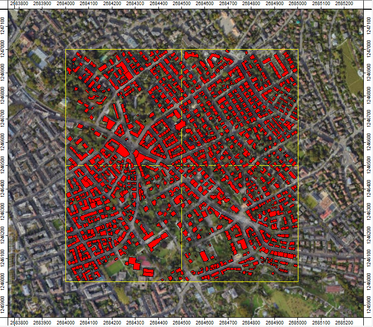
This will create a layer with buildings that are completely contained in the AOI. Right click on the layer in the Data tab and save it to the vector folder as Building_Footprints_Selection
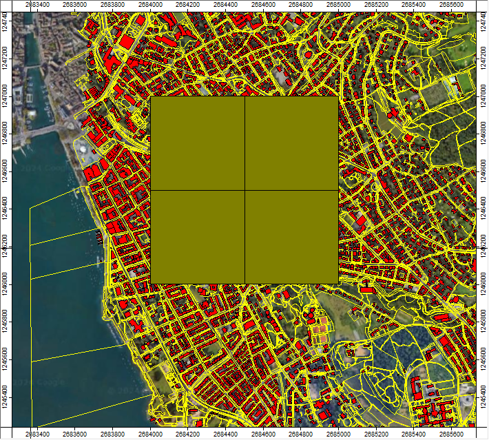
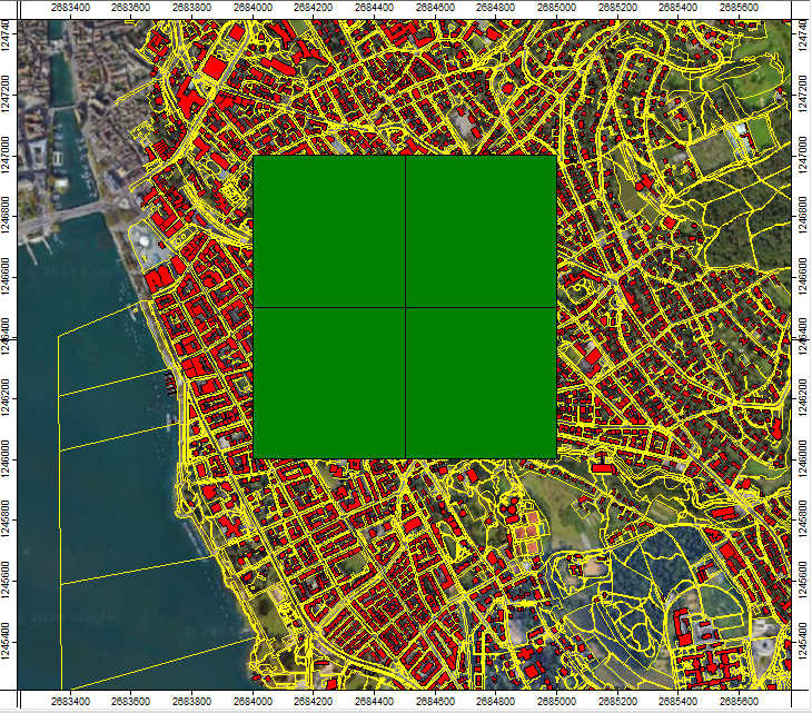
Create Tiling Scheme for Chunk-Wise Processing
Let’s say, we want to process the data in 250x250m chunks. The concept of chunking down the processing into smaller processing units helps in rolling out the procedures for large areas. Let’s create the processing units:
Tool: Create Spatial Processing Units
Geoprocessing → LIS Pro 3D → Tools → Shapes // Tools → LIS Pro 3D → Tools
| Parameter | Setting |
|---|---|
| Data Objects | |
| Shapes | |
| << Units | <create> |
| Options | |
| Extent and Tile Size | |
| > Extent | AOI |
| Round Lower-Left Origin | 🗹 |
| Tile Size | 250 |
| Adaptive Subdivision | |
| Subdivision | none |
- Provide the AOI in the Extent section
- Set Tile Size to 250m
- Click Execute
In the Data Tab a processing_units dataset has been created.
- Rename the it to Proc_Tiling
- Right-click the datasets and click Save as into your vector folder
- Change the Fill Style to Transparent and Outline Color to green
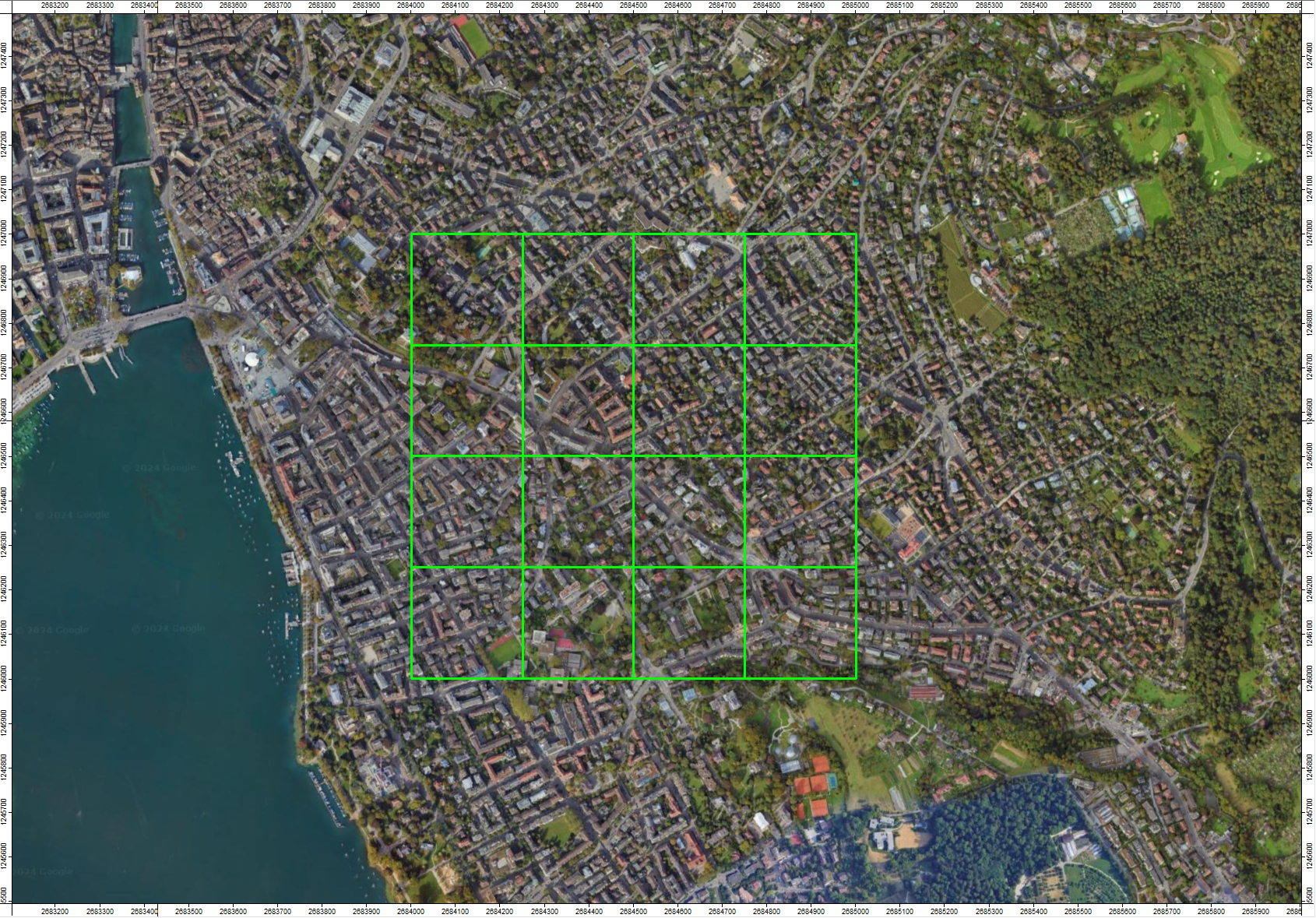
Now we have defined 16 chunks that will be processed independently.