Prepare Processing
< Previous section Next section >
Create a New LIS Pro 3D Project
- Open LIS Pro 3D with an empty project (close any previous project!)
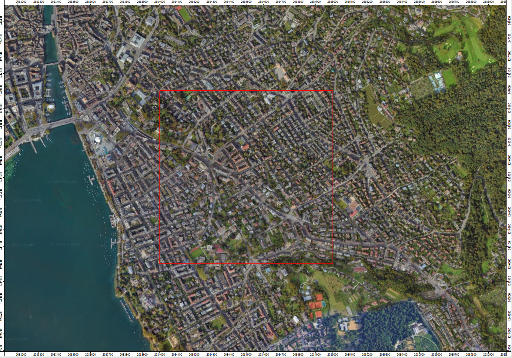
- Use: File > Data > Shapes in order to open the AOI shapefile we have created in the previous tutorial. This is the area that we want to process.
- Set the Fill Style for AOI to Transparent (and the Outline > Color to red)
- Add Google Satellite as a base map to the map
- Use: File > Data > Shapes in order to open the “Proc_Tiling” shapefile we have created in the previous tutorial section. This dataset defines our processing chunks for area-wide processing.
- Add Proc_Tiling to the current map
- Change the Fill Style for Proc_Tiling to Transparent and Outline > Color to green
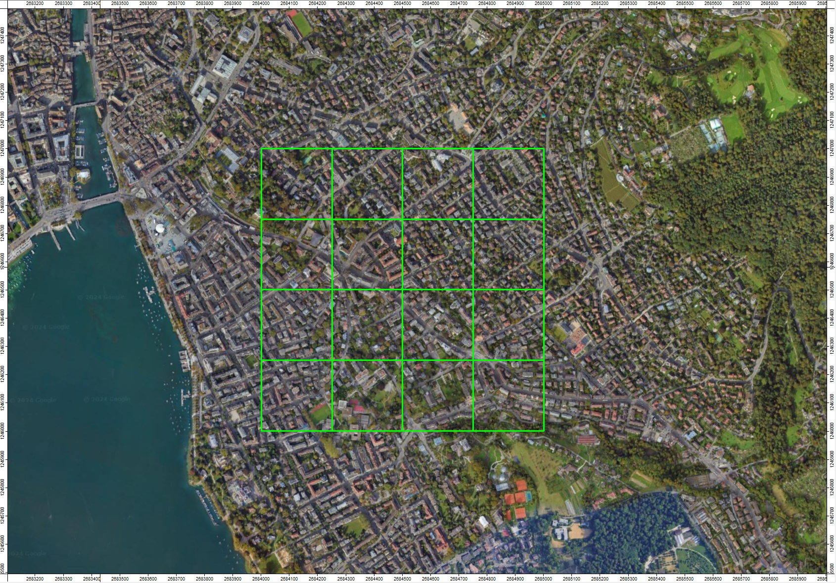
Now we have 16 tiles, which define the processing units of our dataset.
Select a Processing Unit from the Tiling Scheme
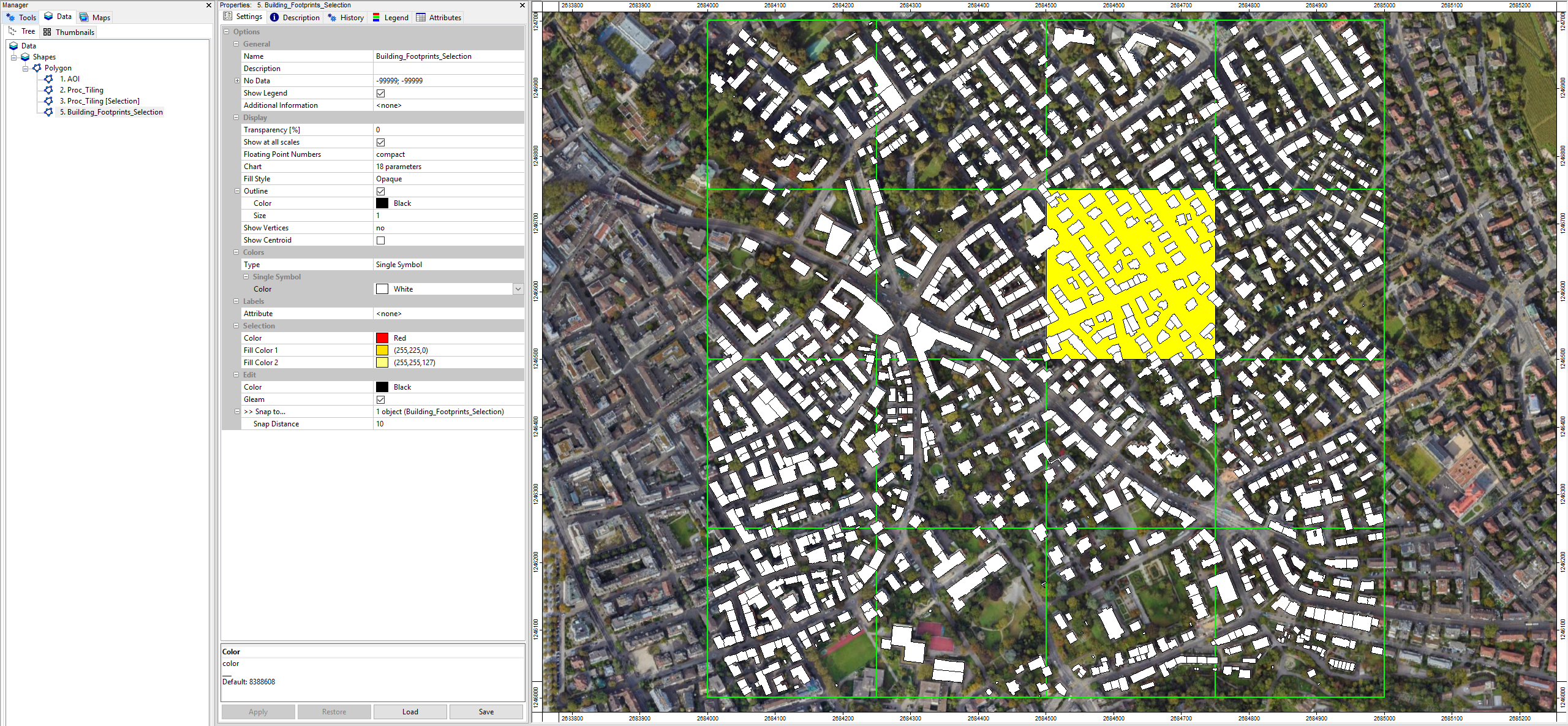
Let’s select a single unit from our tiling scheme for testing.
- In the Data Tab select Proc_Tiling
- Use the Interaction Tool (the interact cursor) in the top menu, and click onto one unit in order to select it
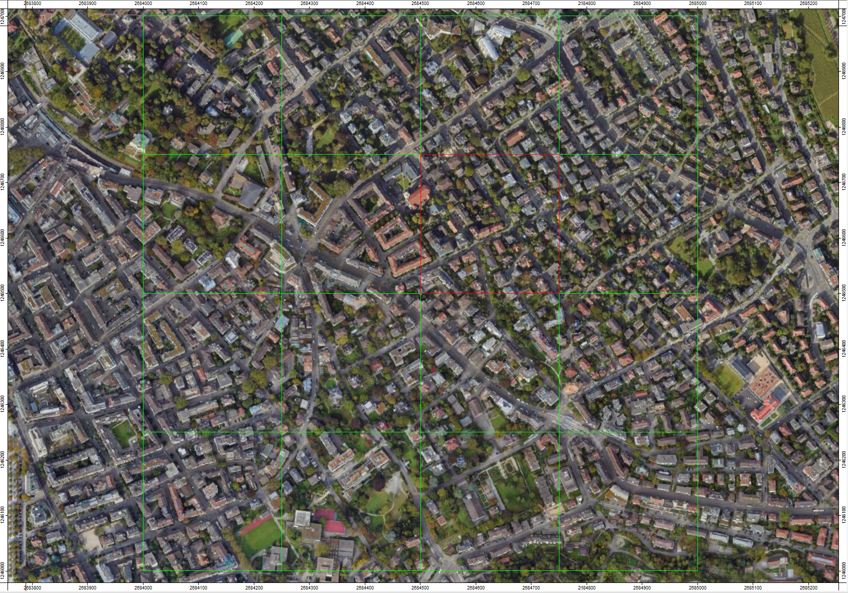
The selected unit is shown in red . Now copy this unit to a new layer:
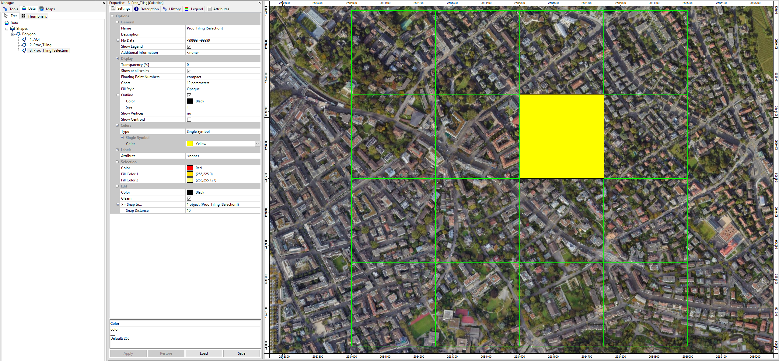
Tool: Copy Selection to New Shapes Layer
Geoprocessing → Shapes → Selection // Tools → Shapes → Tools
| Parameter | Setting |
|---|---|
| Data Objects | |
| Shapes | |
| >> Input | Proc_Tiling |
| << Output | <create> |
- Provide the Proc_Tiling layer
- Click Execute
In the Data Tab a new polygon layer appears. Add it to the map.
Load Prepared Building Footprints
Use: File > Data > Shapes in order to open the Building_Footprints_Selection shapefile we have created in the previous tutorial. Add it to the map.
Find Corresponding Buildings for Selected Unit
Processing the dataset in smaller subsets means we also need to chunk down the buildings into smaller subsets. In this process, we need to ensure that each building is processed exactly once. Additionally, we are not allowed to cut buildings that are located on the boarder of processing chunks. To do so, we associate each building polygon to a specific chunk by the location of its centroid. These centroids always fall into a single unit. Use the tool: Shapes > Tools > Select by Location …:
Tool: Select by Location…
Geoprocessing → Shapes → Selection // Tools → Shapes → Tools
| Parameter | Setting |
|---|---|
| Data Objects | |
| Shapes | |
| >> Shapes to Select From | Building_Footprints_Selection |
| >> Locations | Proc_Tiling [Selection] |
| << Copy | <create> |
| Options | |
| Condition | have their centroid in |
| Method | new selection |
| Post Job | copy |
- Provide the building shape layer as Shapes to Select From
- Provide the current processing unit (Proc_Tiling [Selection]) as Locations
- Use the Condition: “have their centroids in”
- Select Post Job: “copy”
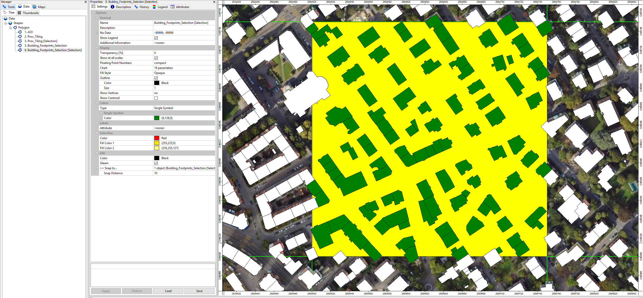
Now we have some buildings that are intersecting with the processing unit, but are not processed, and some buildings that are intersecting with neighboring units but are still considered for the currently selected unit because of having their centroids in the currently selected unit.
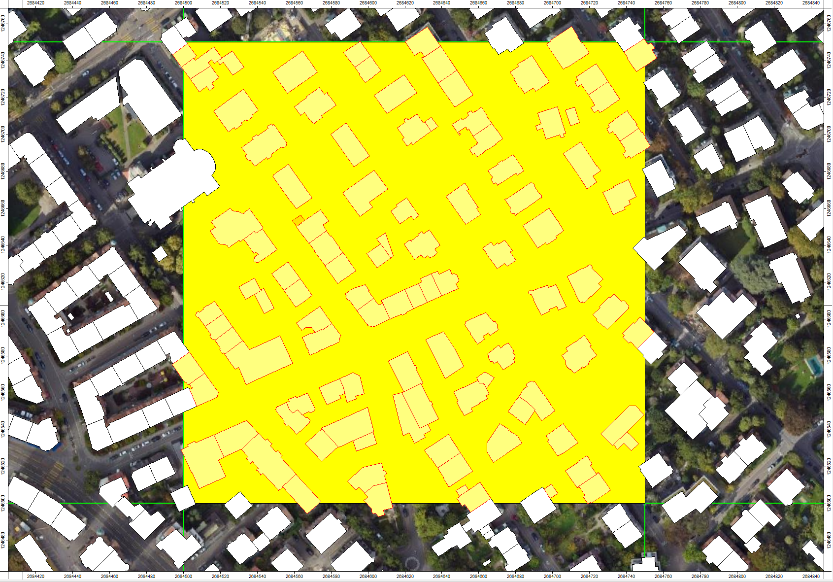
In the Data Tab a new polygon layer with the selected buildings appears (Add it to the map).
Derive the Processing Extent
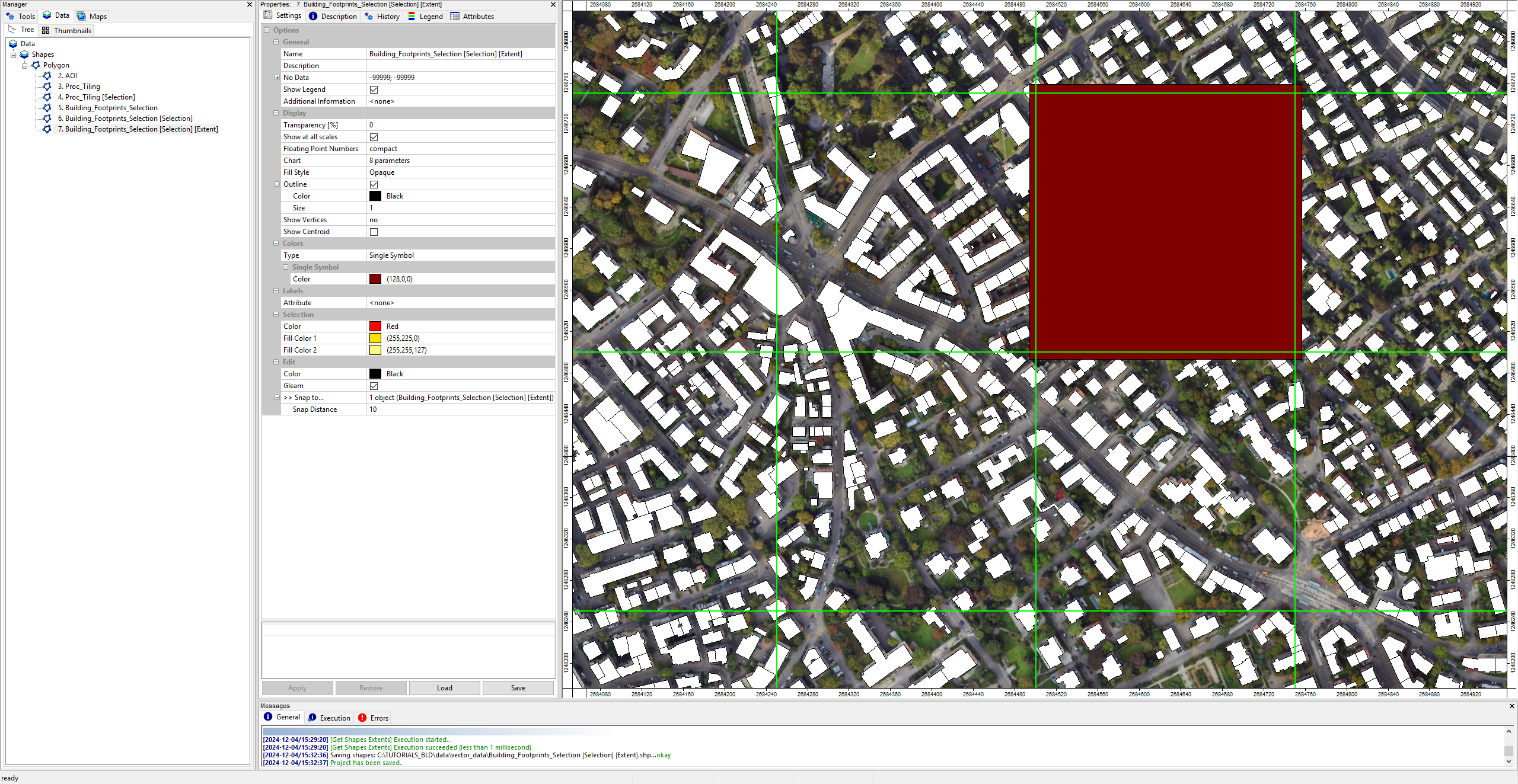
Some buildings associated with the current unit lie only partly within it (i.e., they extend into neighbouring units). If we process the point cloud with the exact bounding box of this processing chunk, we would capture only a part of those buildings. Therefore, we need to expand the unit’s processing extent to fully include the selected buildings! Let’s derive this expanded processing extent for the buildings within the unit:
Tool: Get Shapes Extents
Geoprocessing → Shapes → Tools // Tools → Shapes → Tools
| Parameter | Setting |
|---|---|
| Data Objects | |
| Shapes | |
| >> Shapes | Building_Footprints_Selection [Selection] |
| << Extents | <create> |
| Options | |
| Get Extent for … | all shapes |
| Add Buffer | 0 |
- Provide the layer Building_Footprints_Selection [Selection]
- Choose all shapes in the Get Extent for… section
- Click Execute
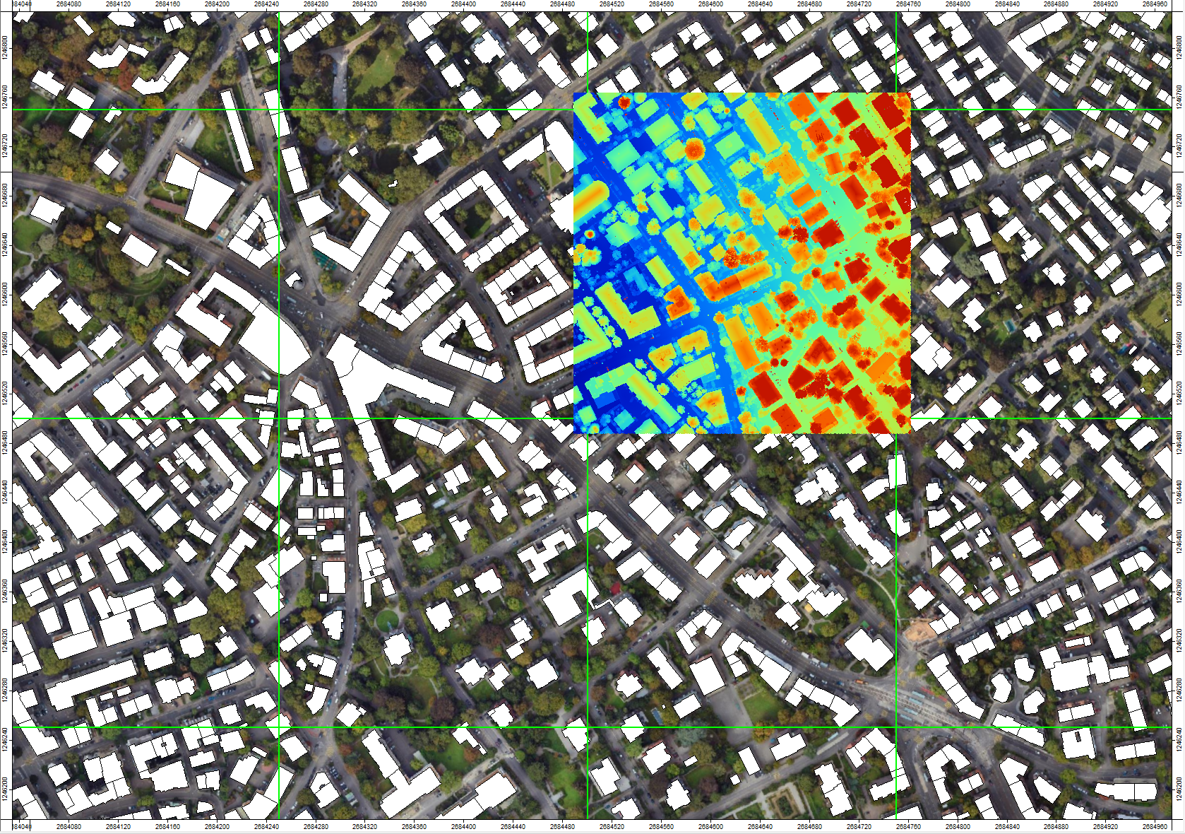
This will create a new layer Building_Footprints_Selection [Selection] [Extent], which is slightly larger than the previous extent of the selected processing unit:
Query and Inspect Point Cloud Subset
Now we can have a look into the available LiDAR data that we have downloaded in the previous section:
Tool: Get Subset from Virtual LAS/LAZ
Geoprocessing → LIS Pro 3D → Virtual → LAS/LAZ // Tools → LIS Pro 3D → Virtual
| Parameter | Setting |
|---|---|
| Options | |
| Filename | C:\\…\lidar\pointclouds\tiles.lasvf |
| Optional Output Filepath | |
| Copy existing Attributes | 🗹 |
| Classes | |
| Last Returns | ☐ |
| Constrain Query | ☐ |
| File Compression | 🗹 |
| Fail on Empty Point Clouds | ☐ |
| Point Cloud Thinning | ☐ |
| AOI | |
| > Shape | Building_Footprints_Selection [Selection] [Extent] |
| Tilename | <not set> |
| Grid system | <not set> |
| > Grid | <not set> |
| X-Extent | 0;0 |
| Y-Extent | 0;0 |
| Add Overlap | 🗹 |
| Overlap | 5 |
| Skip Empty AOIs | ☐ |
| Optional Tile Info Filename | |
| One Point Cloud per Polygon | ☐ |
- Use the browse button to provide the previously created lasvf file in the Filename section
- Provide the extent of the selected building (Building_Footprints_Selection [Selection] [Extent]) in the Shape section
- Check the Add Overlap checkbox and set the Overlap to 5m - just to be absolutely sure that we are not ignoring any relevant data
- Click Execute
This shows that we can create a point cloud for a randomly defined extent, independent from the physical tiling of the original laz-files (in our case 4 files). This point cloud is completely unaffected by the actual, physical tile boundaries and has no visible edge effects.
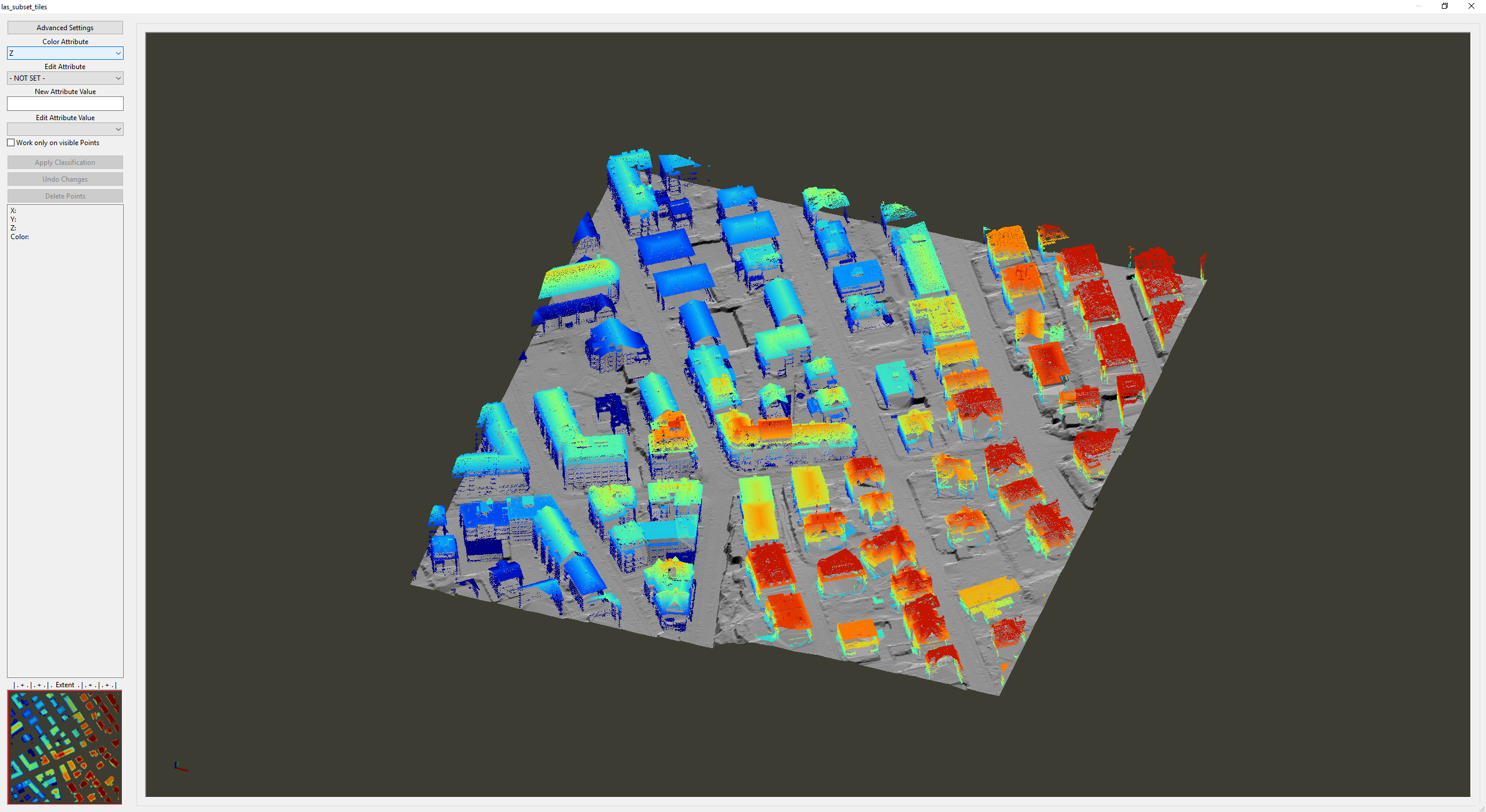
A new point cloud layer las_subset_tiles has been added to the Data Tab. Double-click on it in order to add it to the map.
View Point Cloud in 3D
Use the Point Cloud Editor to inspect the point cloud:
Tool: Point Cloud Editor
Geoprocessing → LIS Pro 3D → Point Cloud Editor // Tools → LIS Pro 3D → Point Cloud Editor
| Parameter | Setting |
|---|---|
| Data Objects | |
| Point Clouds | |
| >> Point Cloud | las_subset_tiles |
| Intensity | intensity |
| RGB | <not set> |
| Shading | <not set> |
| Classification | classification |
| Random | <not set> |
| Normal Vector (X) | <not set> |
| Report Attribute 1 | <not set> |
| Report Attribute 2 | <not set> |
| Grids | |
| > Elevation Grids | No objects |
| > Color Grids | No objects |
| Shapes | |
| > Shapes | <not set> |
| Options | |
| Work on Copy of Point Cloud | ☐ |
| Background Color | Black |
| Classification LUT | ASPRS LAS (Formats 6-10) |
- Provide the las_subset_tiles in the Point Cloud section
- Provide the intensity attribute in the Intensity section
- Provide the classification attribute in the Classification section
- Click Execute
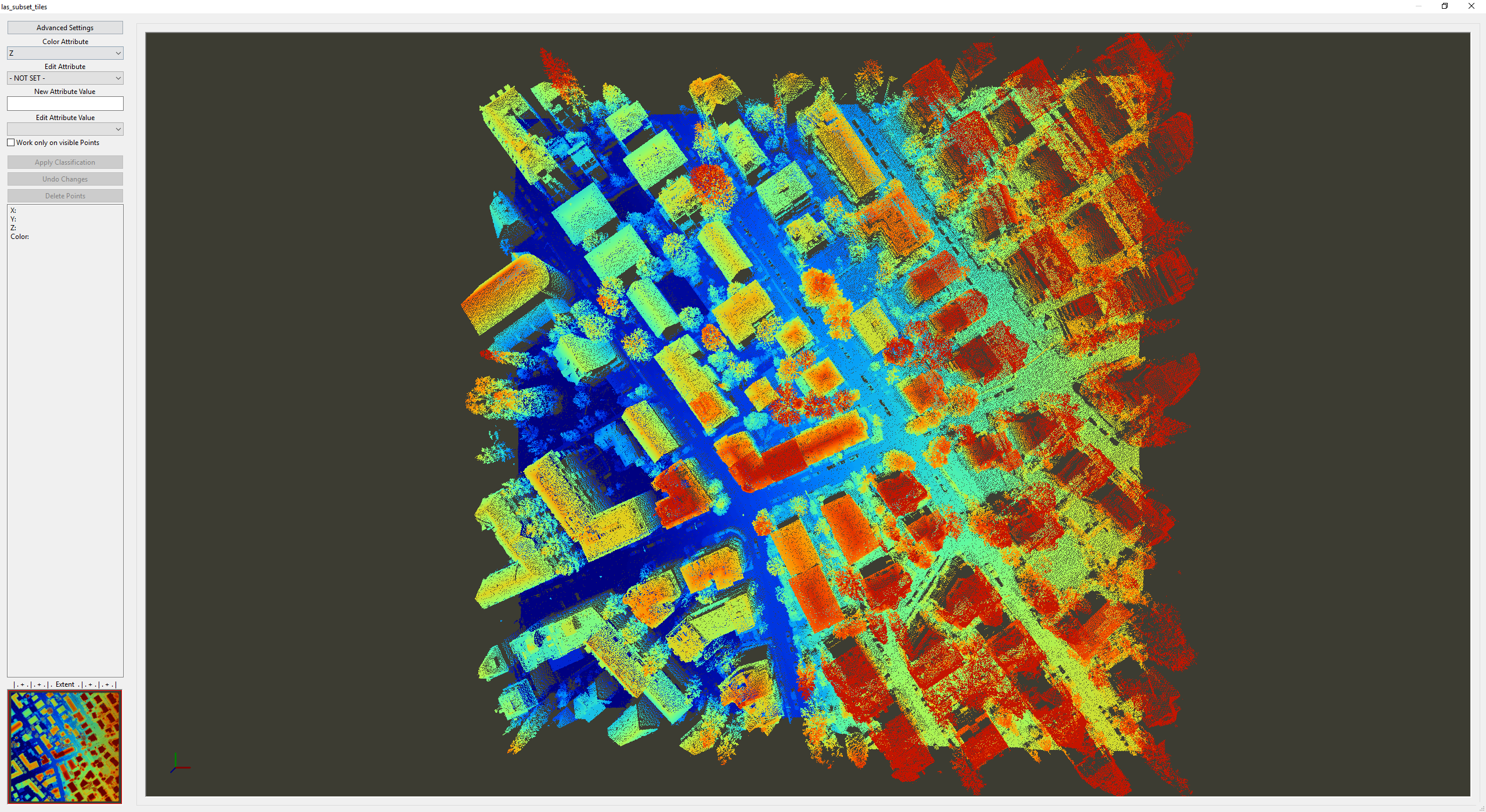
Type 5 in order to switch to classification coloring
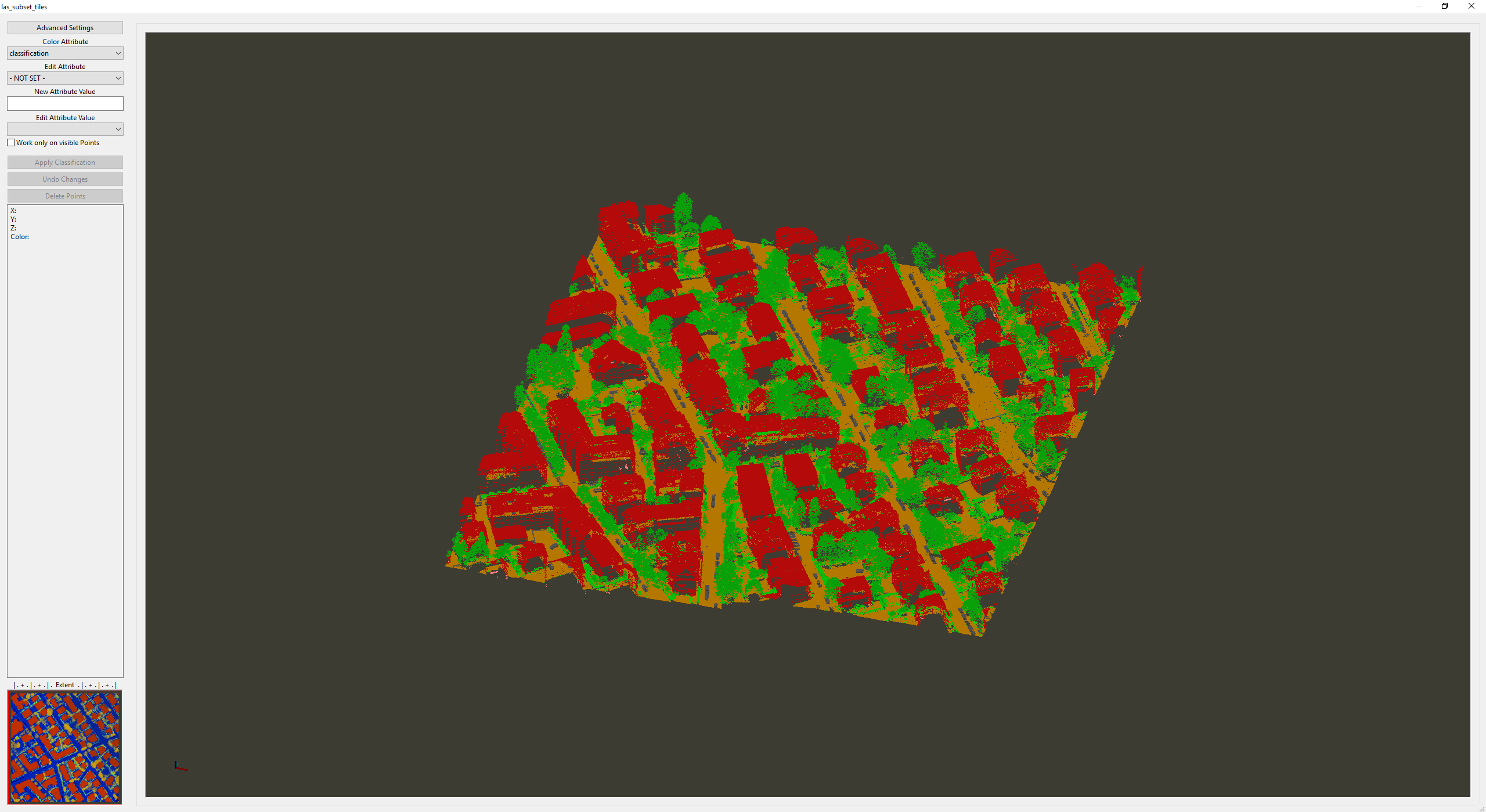
In our case the point cloud is allready classified into, ground, low vegetation, mid vegetation, high vegetation, buildings
Delete Point Cloud Subset
For the reconstruction of building models we don’t need all LiDAR points. We only need to consider building points. Therefore, we can delete the current point cloud subset and query a new subset that only contains building points.
In the Data tab Right-click onto las_subset_tiles and close it.
Query Building Subset from Available Point Cloud Data
Tool: Get Subset from Virtual LAS/LAZ
Geoprocessing → LIS Pro 3D → Virtual → LAS/LAZ // Tools → LIS Pro 3D → Virtual
| Parameter | Setting |
|---|---|
| Options | |
| Filename | C:\\…\lidar\pointclouds\tiles.lasvf |
| Optional Output Filepath | |
| Copy existing Attributes | 🗹 |
| Classes | |
| Last Returns | ☐ |
| Constrain Query | 🗹 |
| Attribute Field | classification |
| Value Range | 6;6 |
| Value List | |
| File Compression | 🗹 |
| Fail on Empty Point Clouds | ☐ |
| Point Cloud Thinning | ☐ |
| AOI | |
| > Shape | Building_Footprints_Selection [Selection] [Extent] |
| Tilename | <not set> |
| Grid system | <not set> |
| > Grid | <not set> |
| X-Extent | 0;0 |
| Y-Extent | 0;0 |
| Add Overlap | 🗹 |
| Overlap | 5 |
| Skip Empty AOIs | ☐ |
| Optional Tile Info Filename | |
| One Point Cloud per Polygon | ☐ |
- Check the Constrain Query checkbox
- Set the Attribute Field to classification
- Set the Value Range to 6;6 (6 is class building)
- Click Execute
Query DTM from Raster Catalog
In the previous tutorial section, we have downloaded official DTMs provided by the Canton of Zurich and created a virtual raster catalog for seamless querying. We will use this DTM in the process of creating building models.
In case you do not have a DTM readily available for your specific use-case, here we provide a step-by-step guide on how to derive a DTM, DSM and nDSM from a point cloud.
Similar to querying the point cloud from the lasvf file (with seamless access independent of the physical tiling), we can query the required extent in the same way from the vrt file (the raster catalog) created in the previous tutorial:
Tool: Import Raster
Geoprocessing → File → Grid // Tools → Import/Export → GDAL/OGR
| Parameter | Setting |
|---|---|
| Options | |
| Input | Files |
| Files | “C:\\…\lidar\DTMs\tiles.vrt” |
| Multiple Bands Output | automatic |
| Select from Multiple Bands | ☐ |
| Transformation | 🗹 |
| Resampling | Nearest Neighbour |
| Extent | shapes extent |
| >> Shapes Extent | Building_Footprints_Selection [Selection] [Extent] |
| Buffer | 5 |
- Provide the previously created vrt file in the Files section
- Choose single grids in the Multiple Bands Output section
- Choose shapes extent in the Extent section
- Provide the extent of the selected building (Building_Footprints_Selection [Selection] [Extent]) in the Shapes Extent section
- Set the Buffer to 5m
- Click Execute
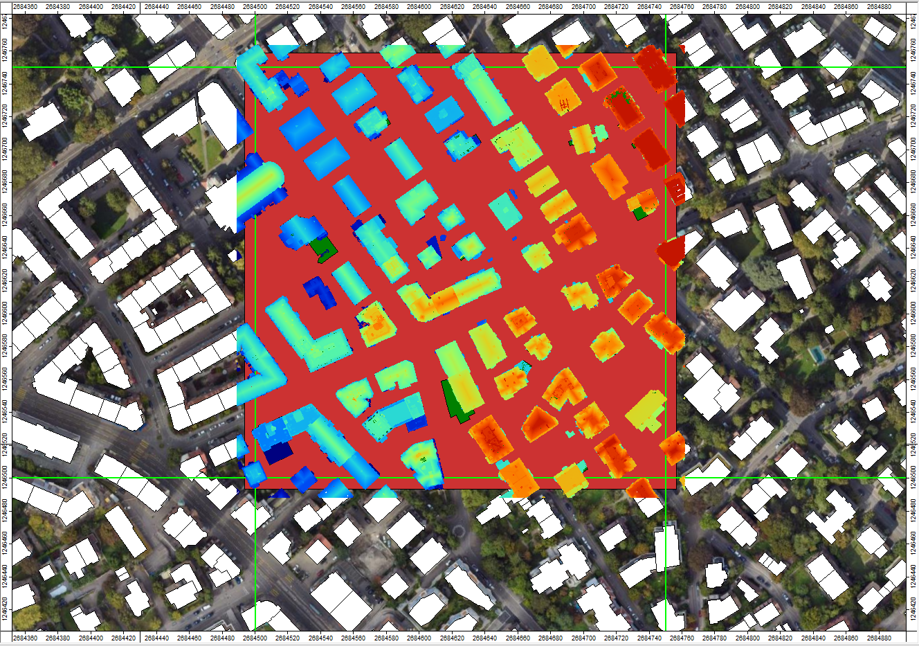
A new grid has been created in the Data Tab. Add it to the map by double clicking:
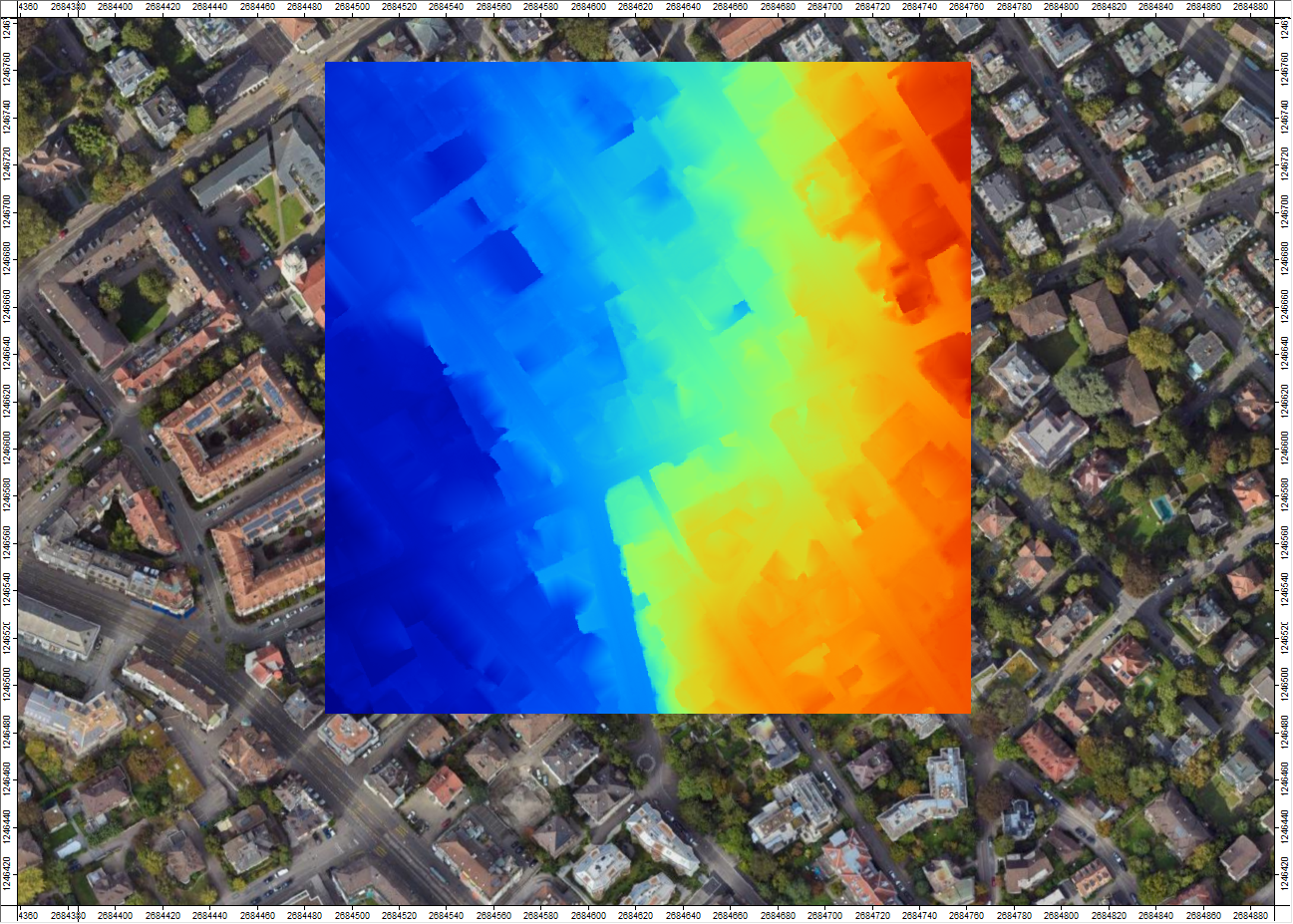
This is the grid that we are going to use in order to create our building models.
Visualization
Create a Hillshade from DTM
Tool: Analytical Hillshading
Geoprocessing → Terrain Analysis → Lighting and Visibility // Tools → Terrain Analysis → Lighting & Visibility
| Parameter | Setting |
|---|---|
| Data Objects | |
| Grids | |
| Grid System | 0.25; 1092x, 1103y; 2684489…x 1246488…y |
| >> Elevation | tiles |
| << Analytical Hillshading | <create> |
| Options | |
| Shading Method | Standard |
| Sun’s Position | azimuth and height |
| Azimuth | 315 |
| Height | 45 |
| Exaggeration | 1 |
| Unit | radians |
- Provide the only available Grid System
- Provide the dataset tiles in the Elevation section
- Click Execute
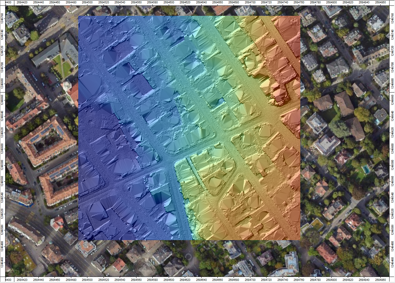
In the Data Tab this creates a new dataset tiles.Hillshade. Add it to the map.
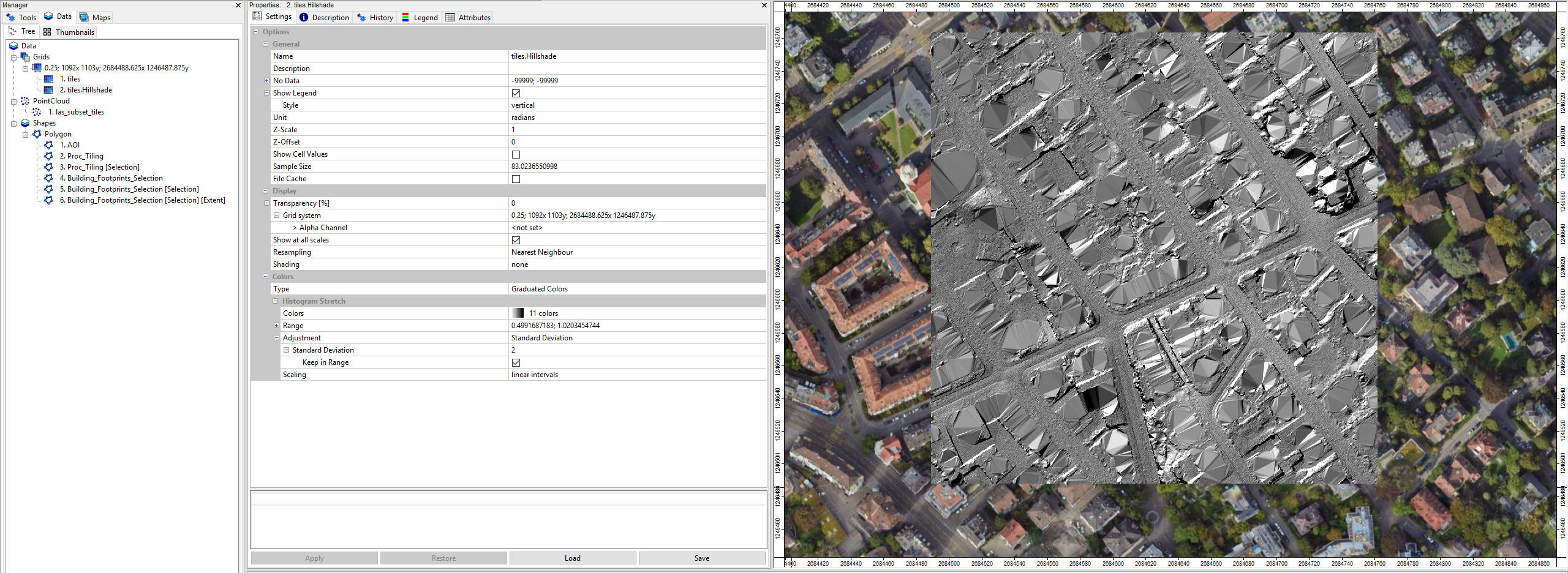
Select the tiles.Hillshade in the Data Tab and in the Object Properties > Settings Tab set the Transparency to 40%:
Visualize DTM and Point Cloud in 3D
Tool: Point Cloud Editor
Geoprocessing → LIS Pro 3D → Point Cloud Editor // Tools → LIS Pro 3D → Point Cloud Editor
| Parameter | Setting |
|---|---|
| Data Objects | |
| Point Clouds | |
| >> Point Cloud | las_subset_tiles |
| Intensity | intensity |
| RGB | <not set> |
| Shading | <not set> |
| Classification | classification |
| Random | <not set> |
| Normal Vector (X) | <not set> |
| Report Attribute 1 | <not set> |
| Report Attribute 2 | <not set> |
| Grids | |
| > Elevation Grids | 1 object (tiles) |
| > Color Grids | 1 object (tiles.Hillshade) |
| Shapes | |
| > Shapes | <not set> |
| Options | |
| Work on Copy of Point Cloud | ☐ |
| Background Color | Black |
| Classification LUT | ASPRS LAS (Formats 6-10) |
- Provide the building point cloud in the Point Cloud section
- Provide the intensity attribute in the Intensity section
- Provide the classification attribute in the Classification section
- Provide the tiles layer in Elevation Grids section
- Provide the tiles.hillshade layer in Color Grids section
- Click Execute
This allows to have a detailed look into the input datasets before processing.
Finally, close the Point Cloud Editor. Save all loaded datasets and save the current project!