Data Preparation for the ALS Forestry Tutorial
Overview
In this tutorial, you will how to extract forestry parameters from an airborne laser scanning dataset. The first step is data preparation - deriving a DEM, DSM and normalized DSM. Once that is done, you can derive a Canopy Height Model (CHM), which allows the detection of single trees and the computation of relevant forestry parameters such as crown area, crown radius, tree height and diameter at breast height (DBH). Finally, the single tree segmentation based on the raster models can be attached to the point cloud dataset, which allows viewing and distinguishing individual trees directly on the point cloud in 3D.
LIS Pro 3D also features a set of dedicated tools that allows single tree reconstruction directly on the point cloud (as opposed to using intermediate raster products), using a bottom-up approach (i.e., 3D segmentation from the stem to the crown). This is especially suited for point clouds acquired by terrestrial laser scanning. The approach allows for computing all relevant forestry parameters. Additionally, it enables the derivation of 3D tree skeleton models, which allow for an even more sophisticated analysis of tree architecture, e.g., regarding branching structure (branching angles, branch size, etc.).
Please refer to our Forestry TLS tutorial if you are interested in this approach.
Data for the ALS Forestry Tutorial
Here you can find two laz-files, which we will use throughout this tutorial. This data is provided by the Canton of Zurich under the CC-BY-4.0 license. Download these two files to follow the tutorial:
2716000_1241000.laz2716500_1241000.laz
Additional Data for the Automation Part (Section 4 & 5)
Additionally, we provide a vector dataset with an area of interest which can be used to follow section 4 & 5 (automation of the forestry analysis):
aoiarea-of-interest.shparea-of-interest...
If you would like to follow the automation guide on forestry analysis, download this dataset as well. Make sure to download all parts of the shapefile (5 individual files).
Please note that some steps in this tutorial require LIS Pro 3D’s Forestry Addon.
Start LIS Pro 3D
Search for LIS Pro 3D in your programs and start it!
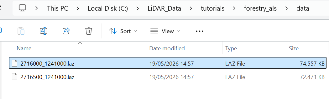
Locate Available Data
In the file explorer of your operating system, search for the downloaded point cloud data. In this example we have two laz files:
Prepare your Data for Processing
Before we load data into LIS Pro 3D, we should perform some preparatory steps that help us accessing the data and performing spatial queries.
It is always recommended to prepare your datasets beforehand, as point clouds usually have large file sizes and can be difficult to handle as single files on a computer.
Create Spatial Index
Now we use the tool Create LAS/LAZ Index in order to create a spatial index for the laz-files!
In all our tutorials, we describe the execution of individual tools via the Tool Libraries interface. If you are not familiar with executing tools this way, please consult this section in our introductory tutorial series. In this section, we describe how you can locate the tools in LIS Pro 3D’s GUI.
Tool: Create LAS/LAZ Index
Geoprocessing: LIS Pro 3D → Import/Export → Create LAS/LAZ Index // Tools → LIS Pro 3D → Import/Export → Create LAS/LAZ Index
| Parameter | Setting |
|---|---|
| Input Files | “/data/2716500_1241000.laz” “/data/2716000_1241000.laz” |
| Input File List | |
| Index All Files | 🗹 |
| Indexing | |
| Tile Size | 0 |
| Threshold | 1000 |
| Adaptive Coarsening | |
| Minimum Point Count | 100000 |
| Maximum Interval Count | -20 |
- Go to the Settings tab in the Properties Window and find the Input Files section.
- Use the browse button in the Input Files section to find your available las/laz files.
- Provide all relevant data to the tool (in this example, the two laz files)
In the lower part of the Tools - Settings you have the following options:
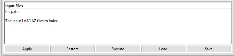
Click Apply, then click Save in order to permanently save the current tool settings.
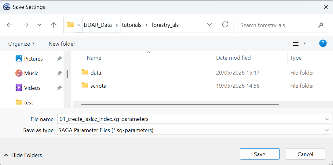
A pop-up window appears, where you can save the currently used setting of the tool into a parameter file (.sg-parameter)
Choose a name (e.g. “01_create_laslaz_index.sg-parameters”) and click Save.
Saving the tool parameters helps to document the different processing steps that have been performed.
Save the parameters for every step you are performing.
After you have saved the current setting, click Execute for this tool
The tool creates spatial indices for each provided las/laz file. This might take some time. The Messages Window will indicate the successfull creation of each index with a dedicated message. This index is written to disk as a new, separate file next to the las/laz files.
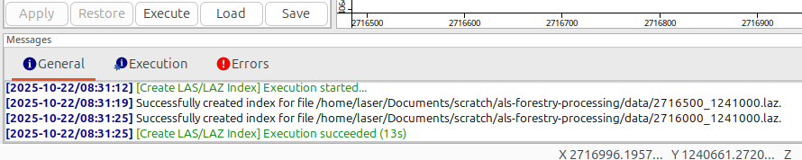
After successfull creation of all indices for the provided las/laz files, a green success message appears in the Messages Window.
Create Virtual Point Cloud Dataset
The following tool creates a so-called virtual point cloud. A virtual point cloud is a concept for treating multiple physical point cloud files (covering e.g. a whole country) as a single point cloud (that only virtually exists). This allows to query parts of the point cloud, independently from the physical tiling of the actual files. The concept avoids border-effects, when selecting data from multiple files. Learn more here
Tool: Create Virtual LAS/LAZ Dataset
Geoprocessing: LIS Pro 3D → Virtual → LAS/LAZ // Tools → LIS Pro 3D → Virtual
| Parameter | Setting |
|---|---|
| Input Files | “ |
| Input File List | |
| Filename | |
| File Paths | relative |
| Color Depth | 16 bit |
| Riegl Extra Bytes | ☐ |
| Ignore LAS File Version | ☐ |
| Ignore Point Data Record Format | ☐ |
| Ignore Coordinate Reference System | ☐ |
- Provide (again) all relevant las/laz files (here: our two tiles) in the Input Files section
- In the Filename section provide the name of the virtual point cloud file (ending on .lasvf) to be created (create it in the same folder as the list!). We here name this file “tiles.lasvf”.
- Click Execute
After this, save the current tool settings (Save).
Get an Overview of Available Data
Now, we are able to get an overview of the available data. Therefore we first create a vector dataset that contains the shape of each las/laz file!
Tool: Create Tileshape from Virtual LAS/LAZ Geoprocessing: LIS Pro 3D → Virtual → LAS/LAZ // Tools → LIS Pro 3D → Virtual
| Parameter | Setting |
|---|---|
| Filename | |
| << Tileshape | <create> |
- Provide the lasvf that we have created in the previous step in the Filename section.
- Click Execute
Note that we are now only using the virtual point cloud (lasvf), ignoring the original list of files!
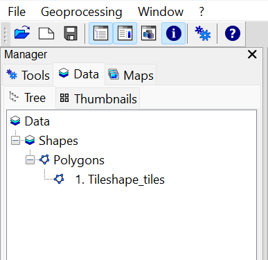
After Execution, a new vector dataset has been created in the graphical user interface. You can find it if you go to the Data tab. By selecting the new layer in the Data tab and selecting the Description tab, you can see the properties of this new layer.
Set Spatial Reference for Layer
To ensure that the projection is defined as intended, manually define the projection for this layer.
Tool: Set Coordinate Reference System
Geoprocessing: Projection // Tools → Projection → PROJ
| Parameter | Setting |
|---|---|
| Options | |
| Definition String | +proj=somerc +lat_0=46.95240555555556 +lon_0=7.439583333333333 +k_0=1 +x_0=2600000 +y_0=1200000 +ellps=bessel +towgs84=674.374,15.056,405.346,0,0,0,0 +units=m +no_defs |
| Display Definition as… | PROJ |
| Authority Code | 2056 |
| Authority | EPSG |
| Geographic Coordinate Systems | <select> |
| Projected Coordinate Systems | <select> |
| Well Known Text File | |
| Pick from Data Set | |
| Customize | |
| Data Objects | |
| Grids | |
| > Grids | No objects |
| Shapes | |
| > Shapes | 1 object (Tileshape_tiles) |
- Provide the Tileshape_tiles in the Shapes section
- Provide the EPSG Code 2056 in the Authority Code section
- Click Execute
The Definition String does not have to be set manually and will be updated automatically with the provided Authority Code.
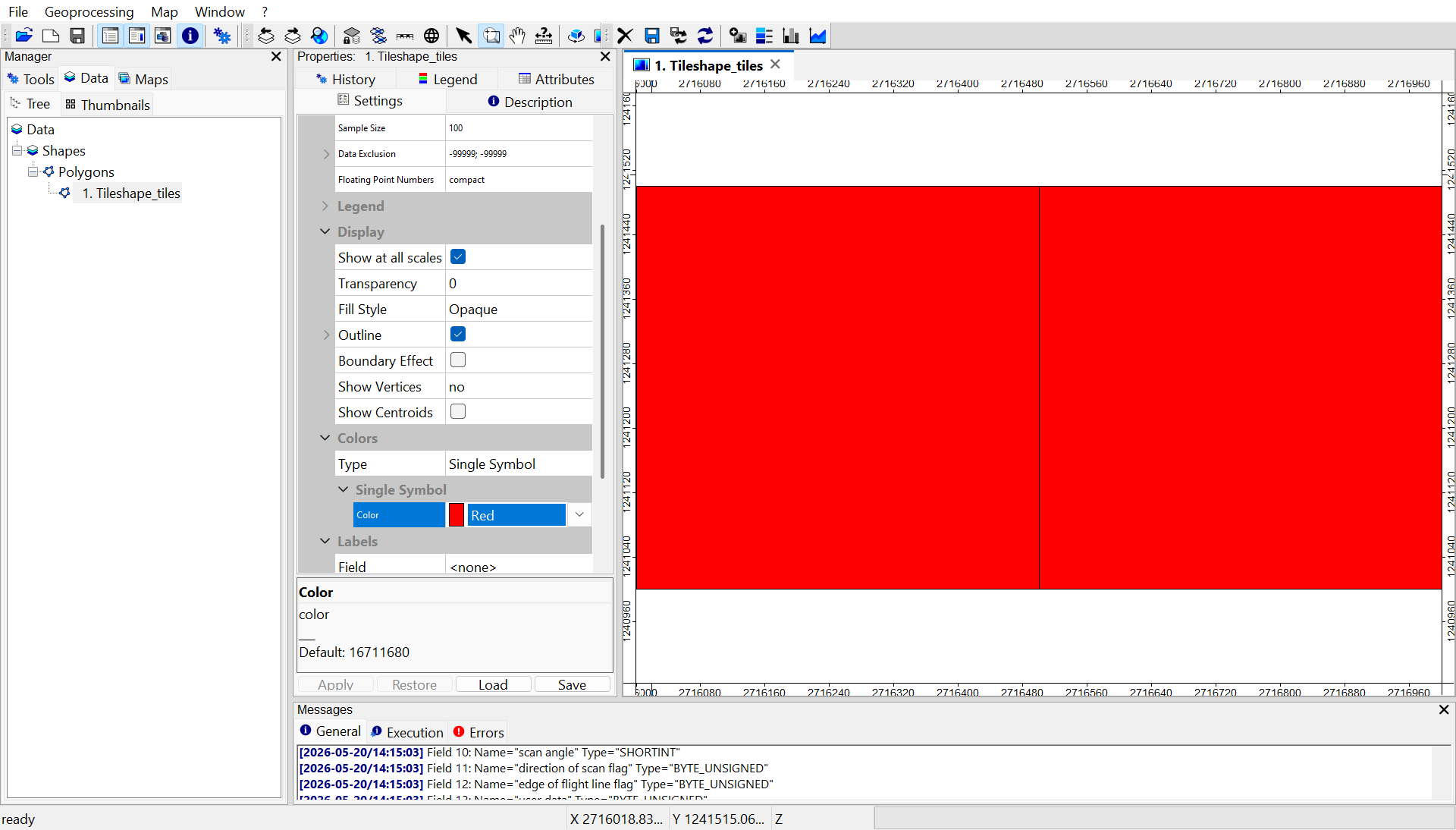
Go to the Data tab again and double click onto the shapes dataset. This will show the dataset in a map.
Add Base Map
Go to the top menu and click onto Map
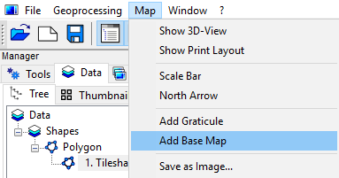
- Select Add Base Map and choose Google Satellite
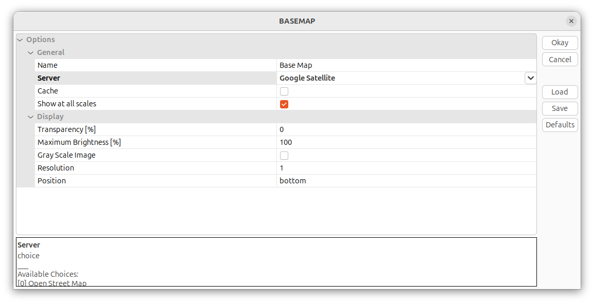
Click Okay, this should load a Base Map to your current map, allowing you to identify, where your available data actually is located.
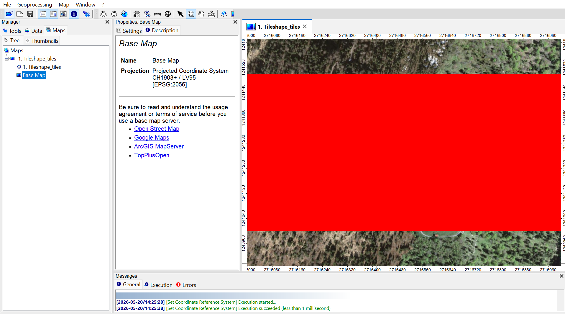
Right-click into the map in order to zoom out:
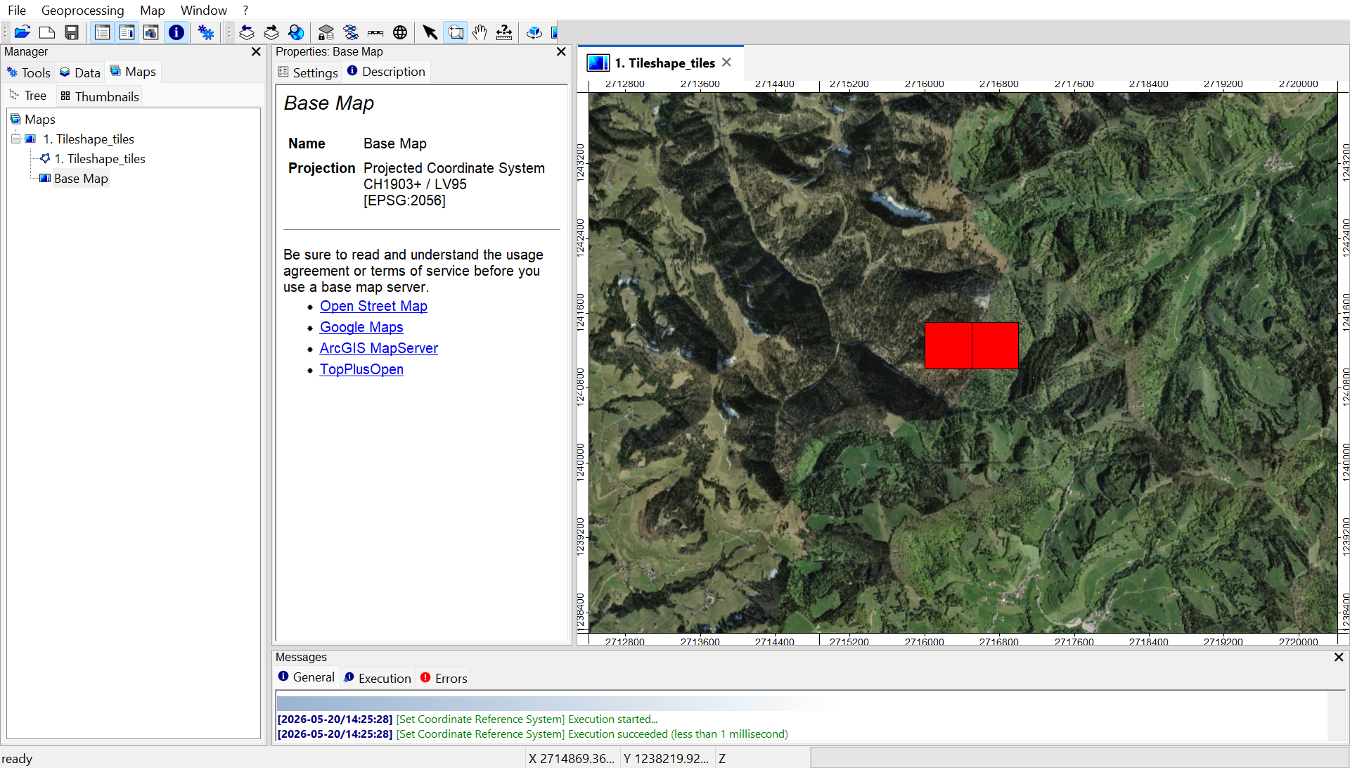
Theoretically, this overview could show an area-wide tile coverage. In this case, we have only two tiles. However, the processing concept is the same for area-wide coverage with thousands of tiles.
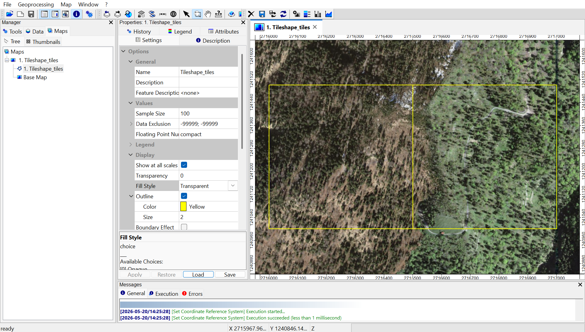
Change View-Type of the Polygon Layer
Select the Tileshape_tiles layer in the Data tab and go to the Settings tab. In the Settings tab you can set:
- Fill Style: Transparent
- Outline > Color: Yellow
- Outline > Size: 2
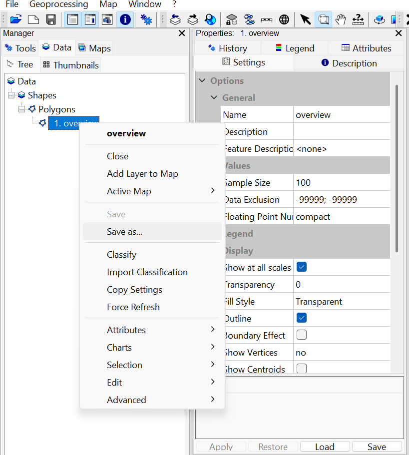
Save Layer to Disk
In the Settings of the shapefile, change the Name to “overview”. Apply this change to the layer. Right-click onto the layer in the Data tab and save the “overview” shapefile to disk using Save as.
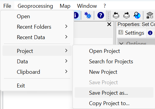
Save Entire Project Permanently
Also save the Project by using the top menu (File > Project > Save Project as…):
It is crucial to save the entire project (and keep it open alltogether) if you would like to continue with the next section of our LIS Pro 3D ALS Forestry tutorial!
Recap
In this tutorial section, we
- Downloaded two files with point cloud data for the Canton of Zurich, Switzerland
- Loaded the point clouds into LIS Pro 3D
- Created a spatial index for the laz-files
- Created a virtual las/laz-file (*.lasvf) - basically a catalog that contains references to our two point clouds
- Created a layer that contains the boundaries of these two point clouds
- Viewed the point cloud extents together with a basemap
- Saved the vector dataset and the project permanently to disk