Point Cloud Visualization and Derivation of Terrain- and Surface Model
< Previous section Next section >
Please make sure that you have completed the previous tutorial, as this section builds upon the previous section!
Open the Project
Open the LIS Pro 3D project that you have saved in the previous section, if you closed LIS Pro 3D in the meantime. Otherwise, simply continue with the opened project.
Query Subset of Point Cloud
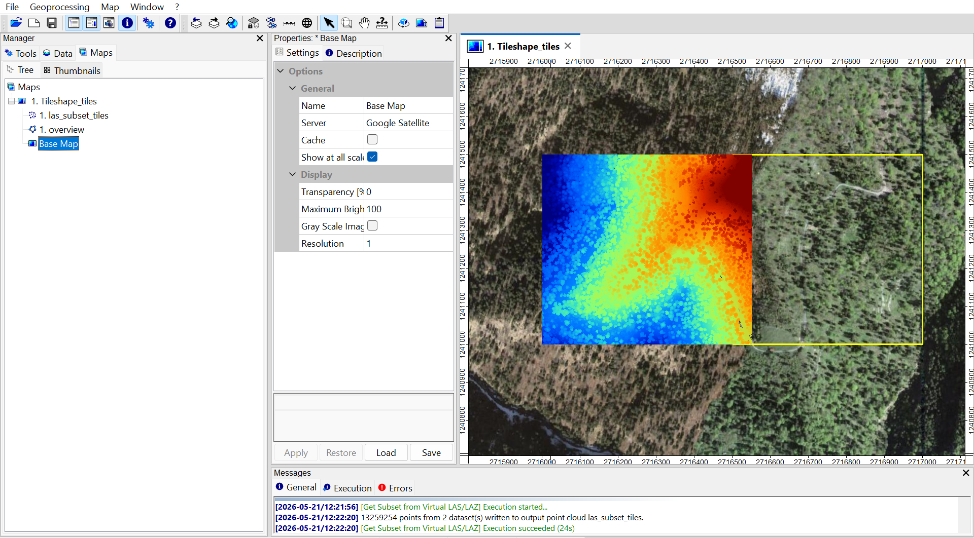
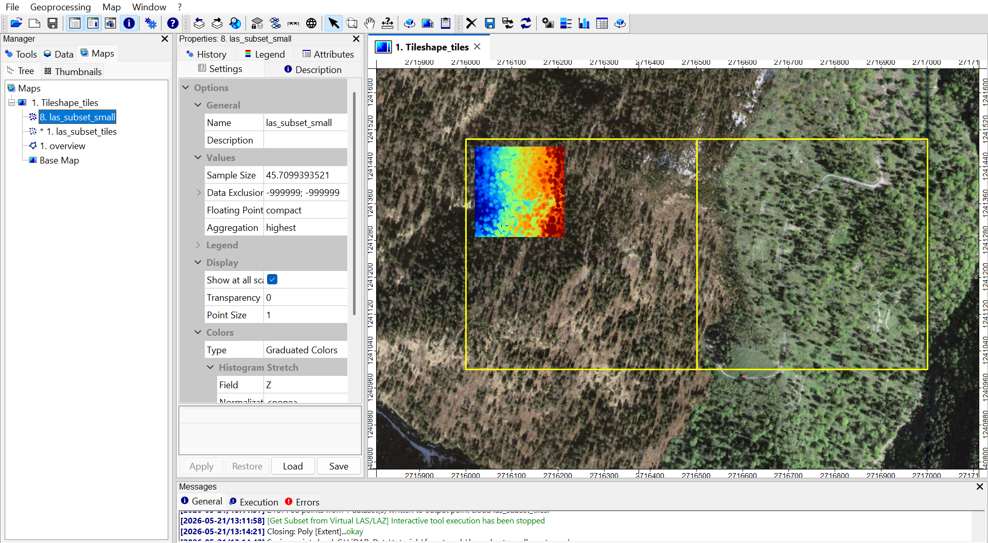
The current map should look similar to this:
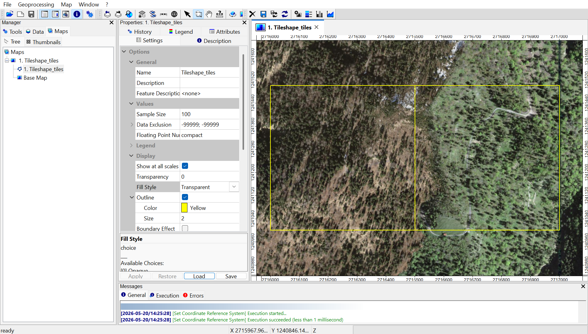
In the Maps tab (inside the Manager Window), click on the overview layer.
This is the prerequsite to enable the interactive selection of individual polygons of a layer in the map view.
Now activate the Interact Tool in the top menu and click into the polygon of interest in order to select it.
Select the left polygon by clicking on it. The selected polygon will get a red border:
With no polygon selected, the following tool would load all point cloud data that is overlapping with one of the two available tiles. In our case we have selected one of the two polygons. With this single polygon selected (in this example 1 out of 2), we can use the given point cloud catalog to query the available point cloud data only within the selected polygon.
Use the following tool to extract a subset from the virtual point cloud:
Tool: Get Subset from Virtual LAS/LAZ
Geoprocessing: LIS Pro 3D → Virtual → LAS/LAZ // Tools → LIS Pro 3D → Virtual
| Parameter | Setting |
|---|---|
| Options | |
| Filename | /data/tiles.lasvf |
| Optional Output Filepath | |
| Copy existing Attributes | 🗹 |
| Classes | 2;3;4;5 |
| Last Returns | ☐ |
| Constrain Query | ☐ |
| File Compression | 🗹 |
| Fail on Empty Point Clouds | ☐ |
| Point Cloud Thinning | ☐ |
| AOI | |
| > Shape | overview |
| Tilename | <not set> |
| Grid system | <not set> |
| > Grid | <not set> |
| X-Extent | 0;0 |
| Y-Extent | 0;0 |
| Add Overlap | 🗹 |
| Overlap | 50 |
| One Point Cloud per Polygon | ☐ |
- Provide the tiles.lasvf in the Filename section
- Provide the Classes we want to load: 2;3;4;5
- Provide the tileshape (here renamed to “overview”) in the Shape section
- Check Add Overlap
- Set Overlap to 50m
- Click Execute
The execution will take some time.
Note that we set a Value Range here. The Value Range includes the classes:
- 2 - ground surface
- 3 - low vegetation
- 4 - mid vegetation
- 5 - high vegetation
It already excludes buildings and all kinds of wires (e.g. powerlines)
Note that we define an overlap of 50m here. For area-wide coverage, this allows selecting a specific tile together with an additional buffer region, in order to avoid edge effects. After the processing, the buffer region is clipped away again.
Learn more about processing with overlap here
In our example, we have only two tiles available, leading to unavoidable edge effects where the data ends. However, at the shared border between the two tiles, we can avoid edge effects by using an overlap.
After successful execution this is indicated in the Messages Window. (

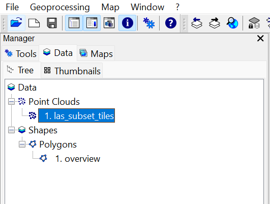
A new point cloud appears in the Data tab.
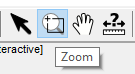
Deselect Interact Tool / Select Zoom Tool
We have made an interactive selection on the tiling scheme, using the Interact Tool. In order to be able to zoom in the map again, select the Zoom tool in the top menu again!
Add Point Cloud to Map
Double Click onto the point cloud in the Data tab.
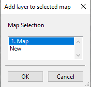
In the pop-up window, choose the existing map (don’t choose New). This will add the queried point cloud to the map.
Query Subset of Point Cloud (interactively)
In the previous step we have queried point cloud data using the selected polygon from the tiling scheme. However, For a quick visualization it might be helpful to select a smaller area. This can be achieved by running “Get Subset from Virtual LAS/LAZ [interactive]”:
Tool: Get Subset from Virtual LAS/LAZ [interactive]
Geoprocessing → LIS Pro 3D → Virtual → LAS/LAZ // Tools → LIS Pro 3D → Virtual
| Parameter | Setting |
|---|---|
| Options | |
| Filename | /data/tiles.lasvf |
| Copy existing Attributes | 🗹 |
| Classes | 2;3;4;5 |
| Last Returns | ☐ |
| Constrain Query | ☐ |
| Clipping Method | lower and left boundary is inside |
| Point Cloud Thinning | ☐ |
| Run Once | 🗹 |
This tool allows an interactive query on our available point cloud data.
Provide the lasvf in the Filename section.
- Provide the tiles.lasvf in the Filename section
- Provide the Classes we want to load: 2;3;4;5
- Provide the tiling scheme (here renamed to “overview”) in the Shape section
- Click Execute
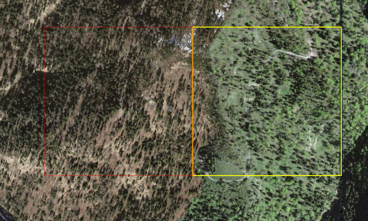
Now the tool waits for user interaction. Therefore we select the Interact tool again.
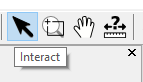
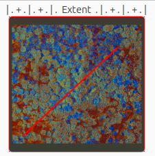
With the Interact tool selected, we select a rectangle in the map:
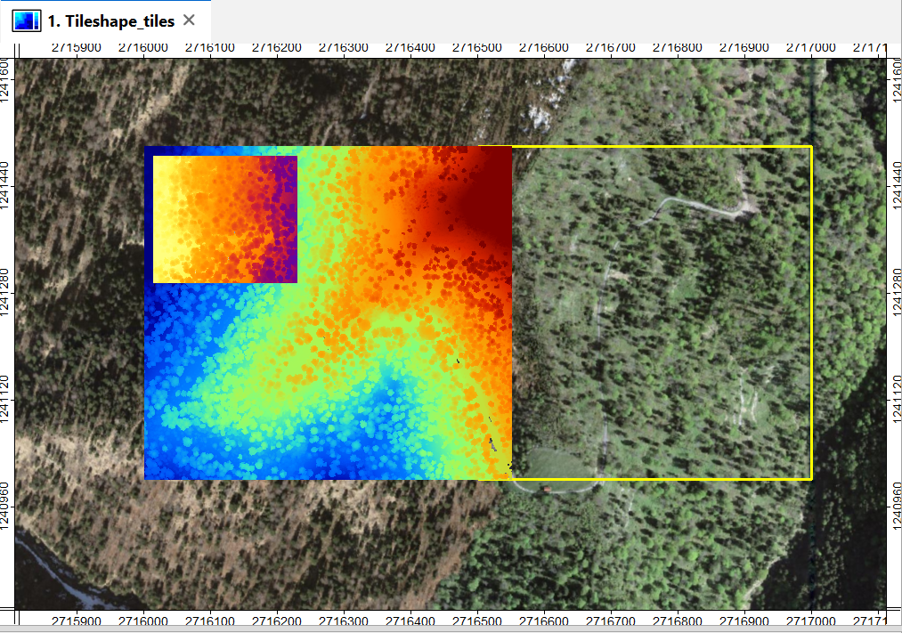
Move your mouse cursor to the upper-left corner of your desired area of interest. Hold the Left-Mouse and drag the diagonal of the rectangle (from the upper-left to the lower-left corner). If you stop holding left mouse the rectangle is accepted and the point cloud query starts. Since the output will be called las_subset_tiles again (as our previous subset), rename it to “las_subset_small”.
The successful execution is indicated in the message window (e.g. 2047222 points from 1 dataset(s) written to output point cloud las_subset_tiles.)
[2025-10-28/07:53:16] [Get Subset from Virtual LAS/LAZ] Execution started...
Interactive tool started and is waiting for user input....
[2025-10-28/07:54:10] 2047222 points from 1 dataset(s) written to output point cloud las_subset_tiles.
[2025-10-28/07:54:10] [Get Subset from Virtual LAS/LAZ] Interactive tool execution has been stoppedDon’t forget to select the Zoom tool again after this operation!
Add Interactively Selected Point Cloud to Map
Add las_subset_small to the map, by double clicking on the layer! Additionally hide las_subset_tiles by double-clicking the layer as otherwise the smaller subset may not be visible.
Save Point Clouds to Disk
In the Data tab, right-click on both point clouds (one after the other, las_subset_tiles, las_subset_small) and save them to disk.
This will save the point clouds as sg-pts-z, which is the native format of LIS Pro 3D.
View (Interactively Selected) Point Cloud in 3D
Use the tool: Point Cloud Editor
Tool: Point Cloud Editor
Geoprocessing → LIS Pro 3D → Point Cloud Editor // Tools → LIS Pro 3D → Point Cloud Editor
| Parameter | Setting |
|---|---|
| Data Objects | |
| Point Clouds | |
| >> Point Cloud | las_subset_small |
| Intensity | intensity |
| RGB | <not set> |
| Shading | <not set> |
| Classification | classification |
| Random | <not set> |
| Normal Vector (X) | <not set> |
| Report Attribute 1 | <not set> |
| Report Attribute 2 | <not set> |
| Grids | |
| > Elevation Grids | No objects |
| > Color Grids | No objects |
| Shapes | |
| > Shapes | <not set> |
| Options | |
| Work on Copy of Point Cloud | ☐ |
| Background Color | (60,60,50) |
| Classification LUT | ASPRS LAS (Formats 6-10) |
- Provide the previously queried point cloud in the Point Cloud section
- Provide the intensity attribute in the Intensity section
- Provide the classification attribute in the Classification section
- Click Execute
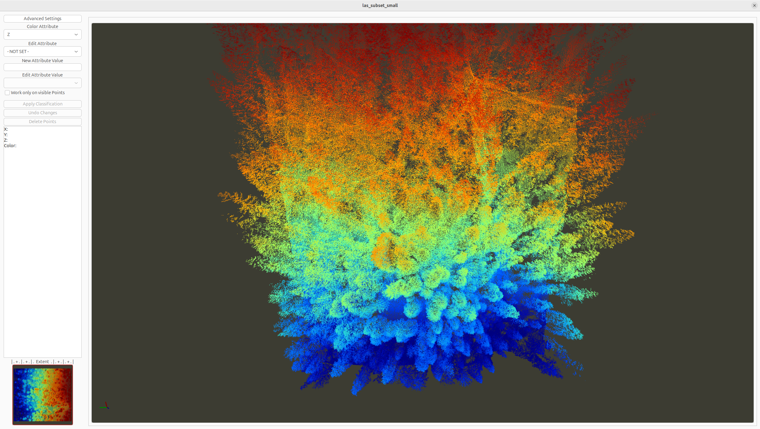
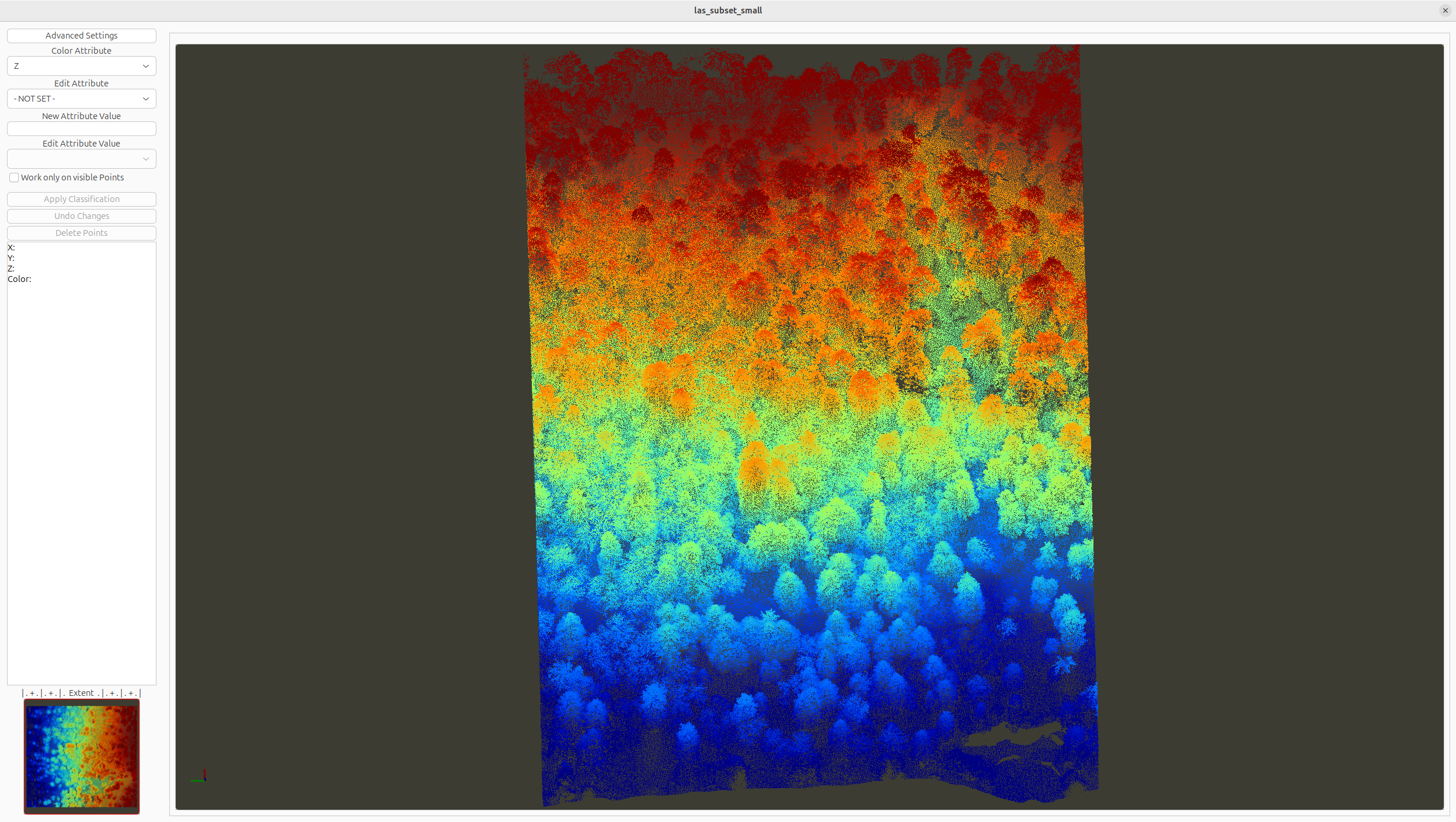
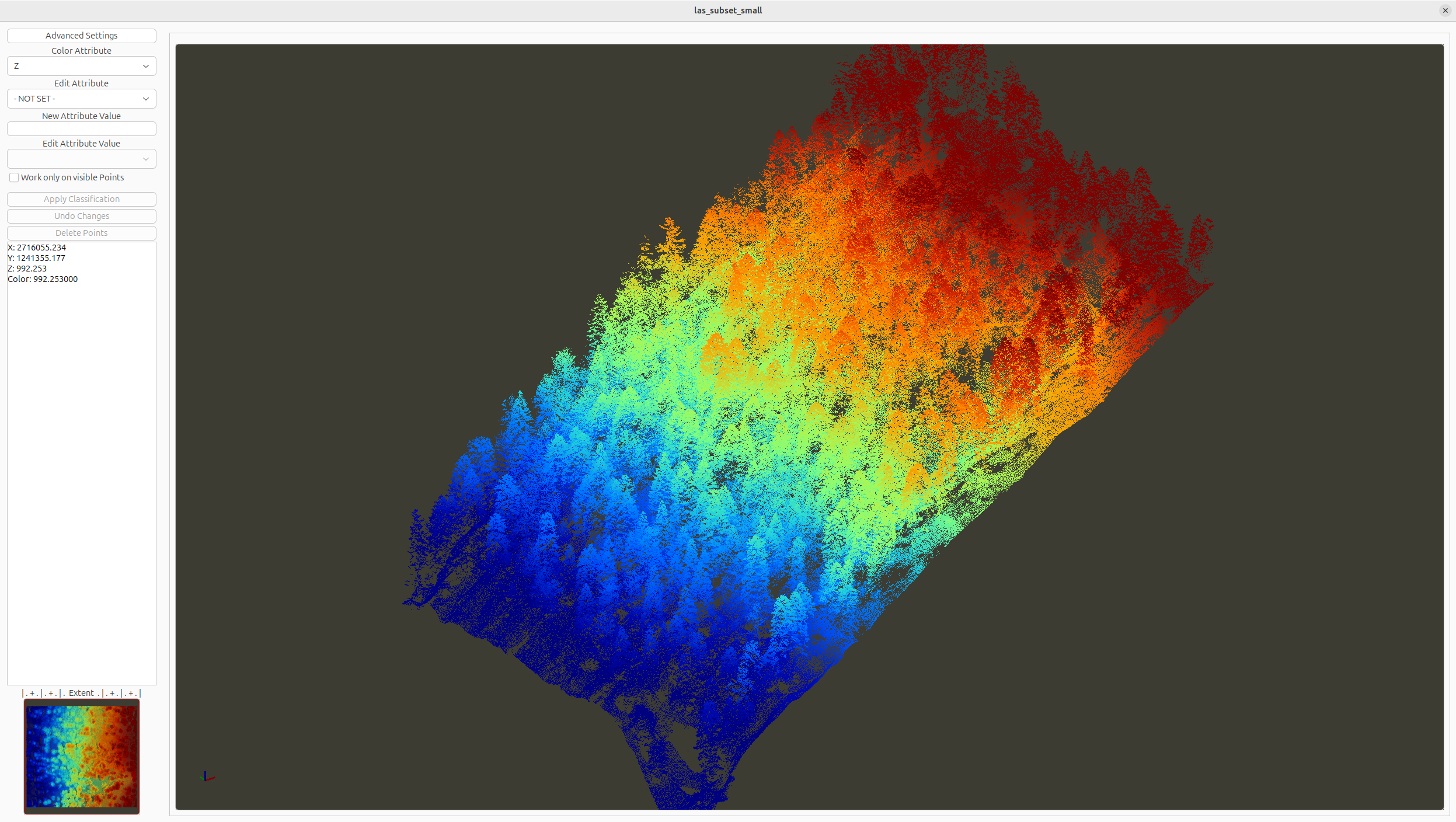
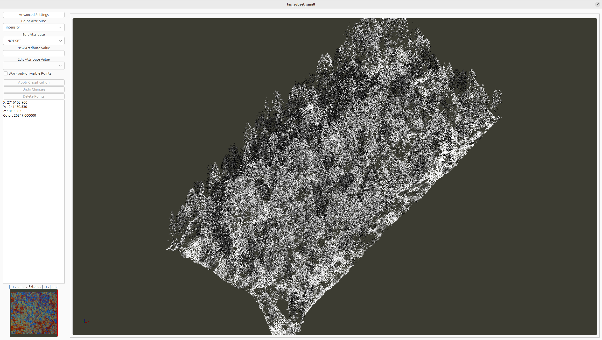
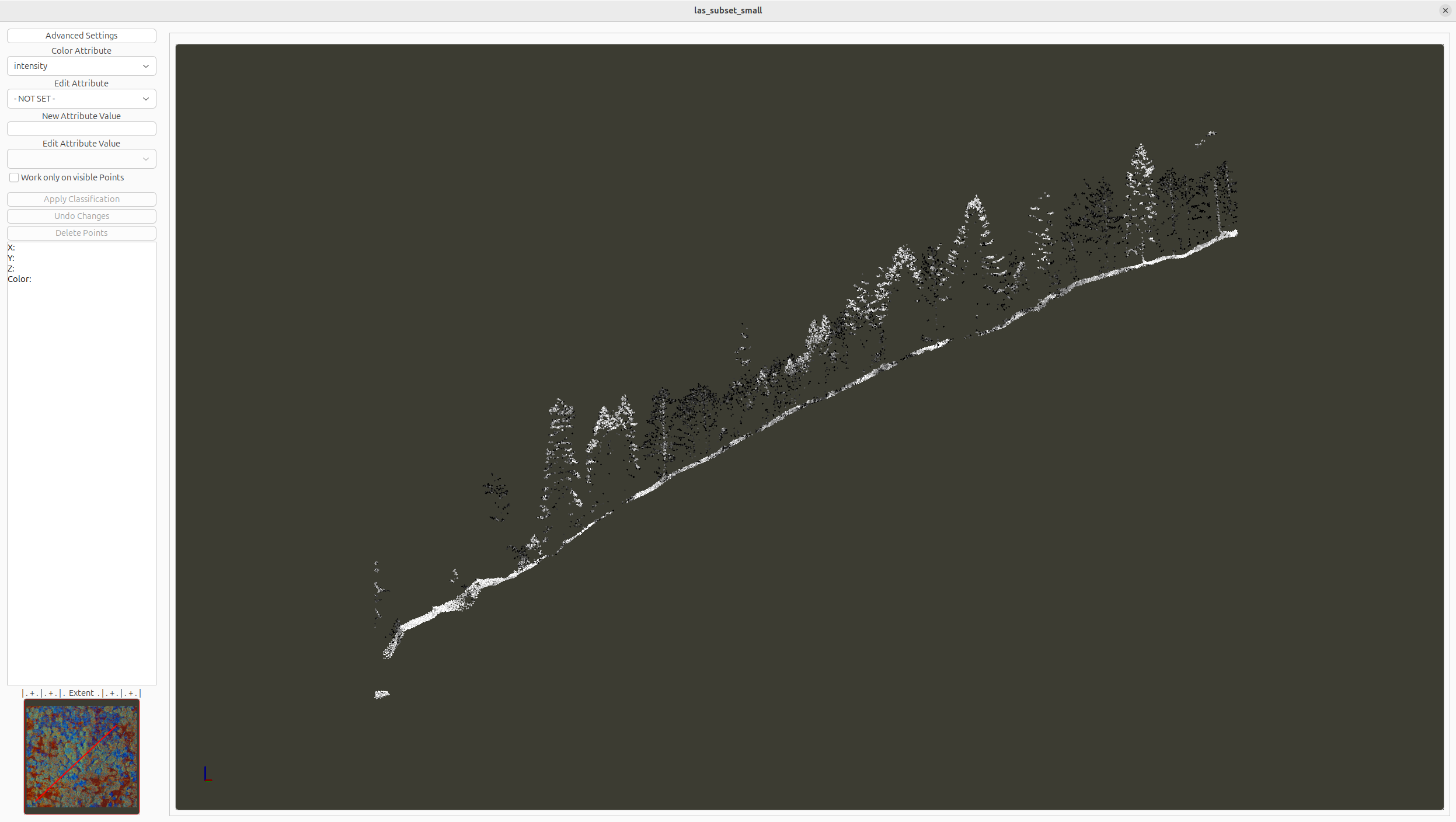
The Point Cloud Editor allows to inspect and edit your point cloud in 3D.
Type: P on the keyboard in order to switch from central projection to parallel projection (and back)
- Hold and move the left mouse, in order turn the point cloud.
- Hold and move the right mouse, in order to move the point cloud sideways.
- Use the scroll wheel, in order to zoom in and out
You can increase the point size by typing F6 on the keyboard and decrease it with F5 again.
You can increase the transparency of the points by typing F12 multiple times on the keyboard and decrease transparency by typing F11 multiple times.
In the moment, the coloring of the point cloud is based on the height values (Z) of the point cloud. (Low values in blue and high values in red).
Type 2 in order to switch to intensity coloring
Type 5 in order to switch to classification coloring
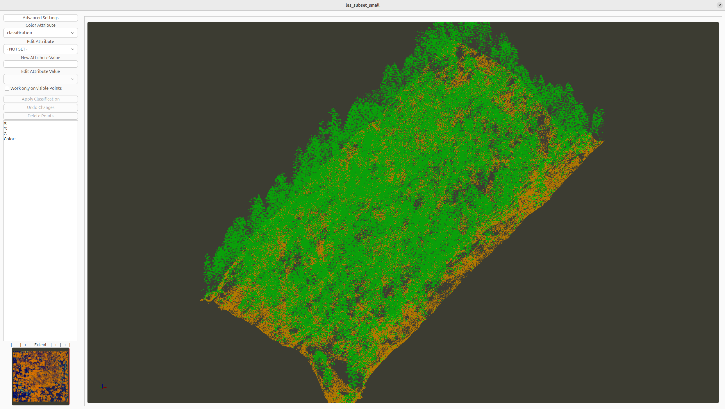
In our case the point cloud is already classified into ground, low vegetation, mid vegetation, high vegetation and buildings
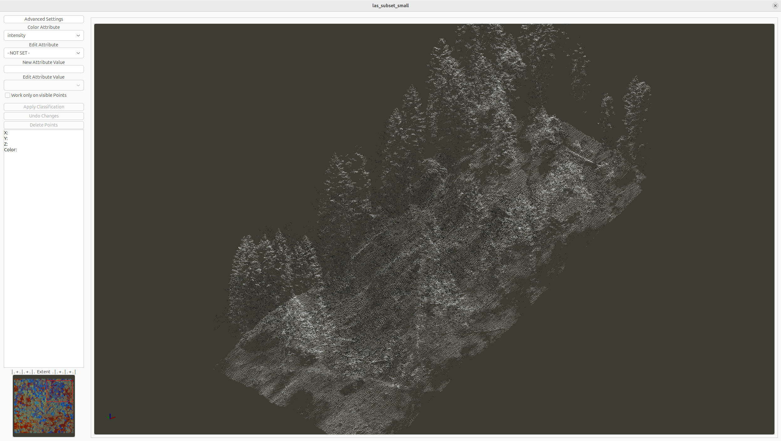
Type 2 again in order to switch back to intensity coloring
Use the lower-left sub map. Drag a rectangle by holding your left mouse, in order to define a sub region (e.g. one single building).
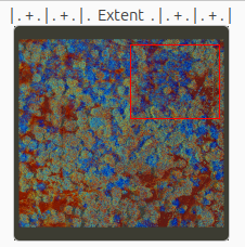
In main view, only the sub region will be visualized and can be inspected in more detail.
Right-click into the sub map, in order to get back the full extent in the main view.
Use the lower-left sub map and drag a line, by holding your right mouse, in order to define a profile through the point cloud. Tip: To improve the visualization, adjust the point size (F5 to decrease/F6 to increase).
Use the upper-right X in order to close the Point Cloud Editor again.
Generate Raster Digital Terrain Model from Point Cloud
Find the tool: LIS Pro 3D > Conversion > Point Cloud to Grid
Tool: Point Cloud to Grid
Geoprocessing → LIS Pro 3D → Conversion → From Point Cloud // Tools → LIS Pro 3D → Conversion
| Parameter | Setting |
|---|---|
| Data Objects | |
| Point Clouds | |
| >> Point Cloud | las_subset_tiles |
| Attribute | Z |
| Filter Attribute | classification |
| Options | |
| Aggregation | mean |
| Attribute Filter | ☐ |
| Elevation Filter | ☐ |
| Search Radius | ☐ |
| Filter Attribute Min / Max | 2;2 |
| Target Grid System | user defined |
| Cellsize | 0.5 |
| West | 2.716e+06 |
| East | 2.7165e+06 |
| South | 1.241e+06 |
| North | 1.2415e+06 |
| Columns | 1001 |
| Rows | 1001 |
| Rounding | 🗹 |
| Fit | nodes |
- Provide the las_subset_tiles in the Point Cloud section.
- Provide the classification attribute in the Filter Attribute section.
Providing the Filter Attribute will apply the Filter Attribute Min/Max Range to the point cloud while generating the raster. In this case it is set to 2;2 (which allows only points labelled as ground points to be selected for gridding).
- Set Aggregation to mean
- Set Target Grid System (user defined) > Cellsize to 0.5 [m]
- Click Execute
A new raster layer appears in the Data tab.
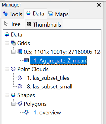
Double click on it, in order to add it to the map.
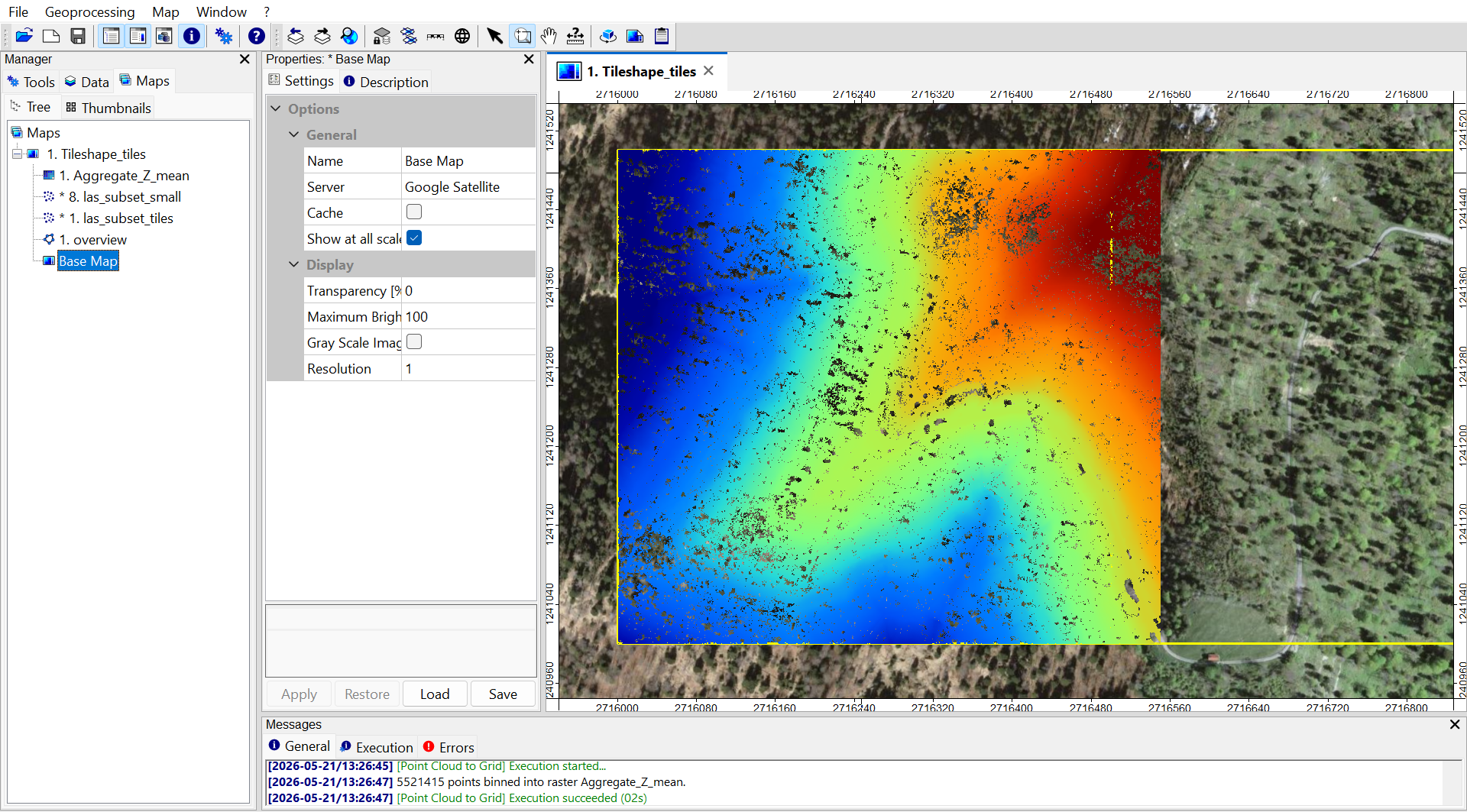
The Basemap can sometimes slow down the renderinmg of the map. Therefore, hide the basemap in the map in order to improve responsiveness.
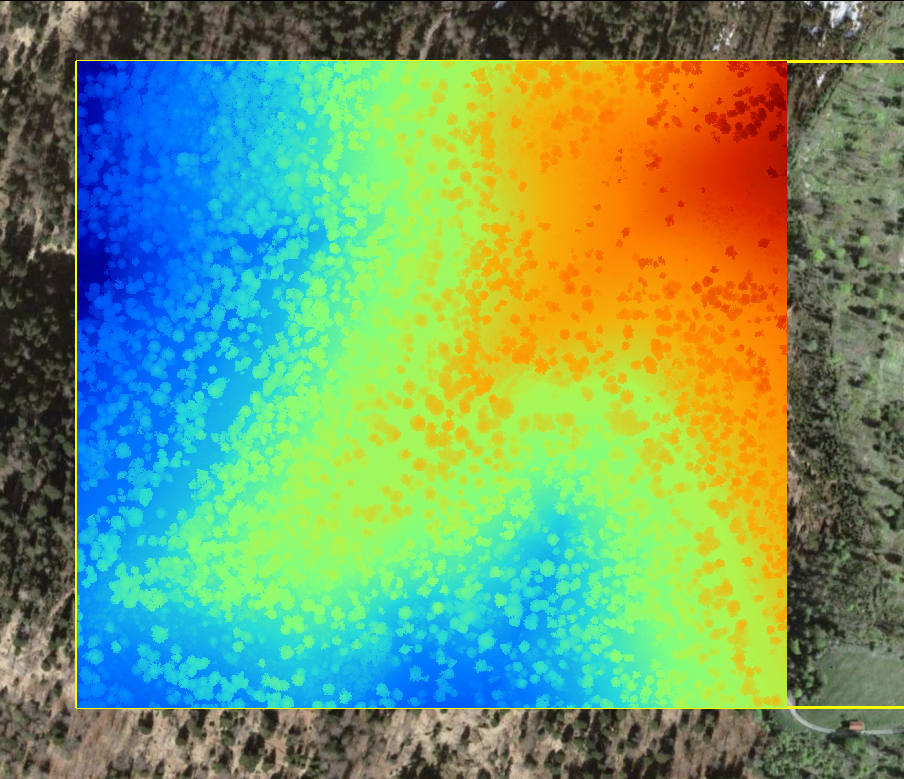
Close Gaps in the Terrain Model
As you can see, the raster dataset is not completely closed. This is a typical scenario for LiDAR flights. Although able to penetrate through canopy, not all laser beams are able to penetrate to the ground. That’s why some areas of the forest floor are not captured.
Find the tool: Grid > Tools > Close Gaps
Tool: Close Gaps
Geoprocessing → Grid → Gaps // Tools → Grid → Tools
| Parameter | Setting |
|---|---|
| Data Objects | |
| Grids | |
| Grid System | 0.5; 1001x, 1001y; 2716000…x 1241000…y |
| >> Grid | Aggregate_Z_mean |
| > Mask | <not set> |
| < Changed Grid | Aggregate_Z_mean |
| Options | |
| Tension Threshold | 0.1 |
- Provide the only available Grid System
- Provide the previously created raster dataset in the Grid section
- Click Execute
This will iteratively close the given Grid and update it. In the Data tab, click on the dataset. Then, in the Object Properties, rename this dataset to DTM.
In the Data tab, right click on the DTM and save it using Save as. Save the dataset as DTM.tif.
Generate Raster Digital Surface Model from Point Cloud
Find the tool: LIS Pro 3D > Conversion > Point Cloud to Grid
Tool: Point Cloud to Grid
Geoprocessing → LIS Pro 3D → Conversion → From Point Cloud // Tools → LIS Pro 3D → Conversion
| Parameter | Setting |
|---|---|
| Data Objects | |
| Point Clouds | |
| >> Point Cloud | las_subset_tiles |
| Attribute | Z |
| Filter Attribute | <not set> |
| Options | |
| Aggregation | max |
| Attribute Filter | ☐ |
| Elevation Filter | ☐ |
| Search Radius | ☐ |
| Target Grid System | grid or grid system |
| Grid System | 0.5; 1001x, 1001y; 2716000…x 1241000…y |
| << Target Grid | <create> |
- Provide las_subset_tiles in the Point Cloud section.
Don’t provide the classification attribute in the Filter Attribute section (leave not set)
- Select Aggregation = max.
- Set Target Grid System to grid or grid system.
- provide the existing Grid System.
- Set Target Grid to create.
This will use the same grid system for the creation of the currently created grid.
- Click Execute
A new raster layer appears in the Data tab. Again, rename this new dataset to DSM and save the dataset to disk as before (right click, …).
Add it to the map!
Close Gaps in the Surface Model
Now we will also close the gaps in the DSM.
Find the tool: Grid > Tools > Close Gaps
Tool: Close Gaps
Geoprocessing → Grid → Gaps // Tools → Grid → Tools
| Parameter | Setting |
|---|---|
| Data Objects | |
| Grids | |
| Grid System | 0.5; 1001x, 1001y; 2716000…x 1241000…y |
| >> Grid | DSM |
| > Mask | <not set> |
| < Changed Grid | DSM |
| Options | |
| Tension Threshold | 0.1 |
You can use the same settings that we used for the DTM, but use the DSM instead.
Save the dataset as DSM.tif.
Generate Normalized Digital Surface Model
Find and run the tool Create nDSM
Tool: Create nDSM
Geoprocessing → LIS Pro 3D → Arithmetic → Grid // Tools → LIS Pro 3D → Arithmetic
| Parameter | Setting |
|---|---|
| Data Objects | |
| Grids | |
| Grid System | 0.5; 1001x, 1001y; 2716000…x 1241000…y |
| >> DSM | DSM |
| >> DTM | DTM |
| << nDSM | <create> |
| Options | |
| Negative Values | set to zero |
- Provide the only available Grid System
- Provide the DSM
- Provide the DTM
- Set Negative Values to set to zero
- Click Execute
This will generate a new nDSM layer, where the canopy height is stored per pixel.
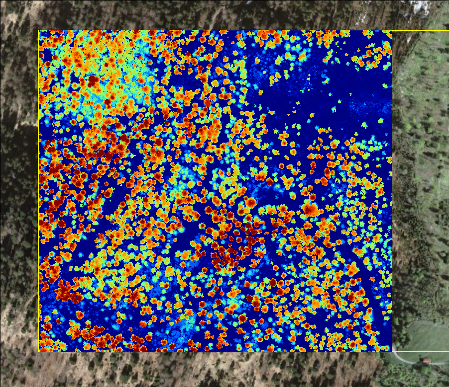
Save the dataset as nDSM.tif.
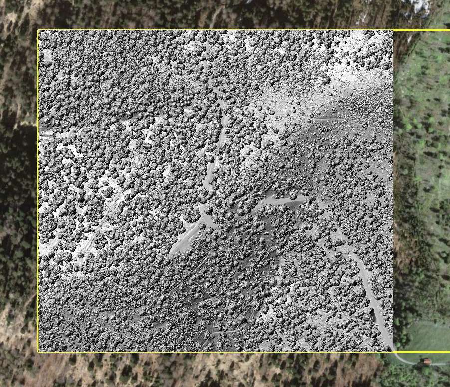
Generate a Hillshade
To achieve more plasticity in the representation, we will generate a hillshade for the DSM
Find the tool:
Tool: Analytical Hillshading
Geoprocessing → Terrain Analysis → Lighting and Visibility // Tools → Terrain Analysis → Lighting & Visibility
| Parameter | Setting |
|---|---|
| Data Objects | |
| Grids | |
| Grid System | 0.5; 1001x, 1001y; 2716000…x 1241000…y |
| >> Elevation | DSM |
| << Analytical Hillshading | <create> |
| Options | |
| Shading Method | Standard |
| Sun’s Position | azimuth and height |
| Azimuth | 315 |
| Height | 45 |
| Exaggeration | 1 |
| Unit | radians |
- Provide the only available Grid System
- Provide the DSM
- Click Execute
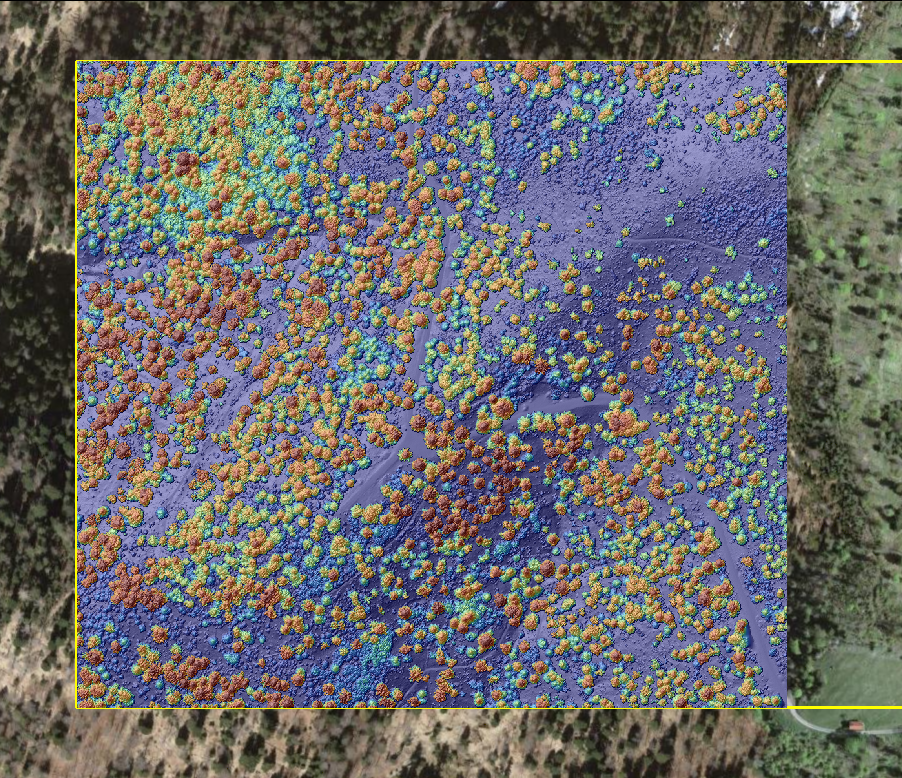
Save the dataset as Hillshade.tif. Add the hillshade to the map. The result will look like this:
In the Settings of the Hillshade Layer, set the Transparency to 40%.
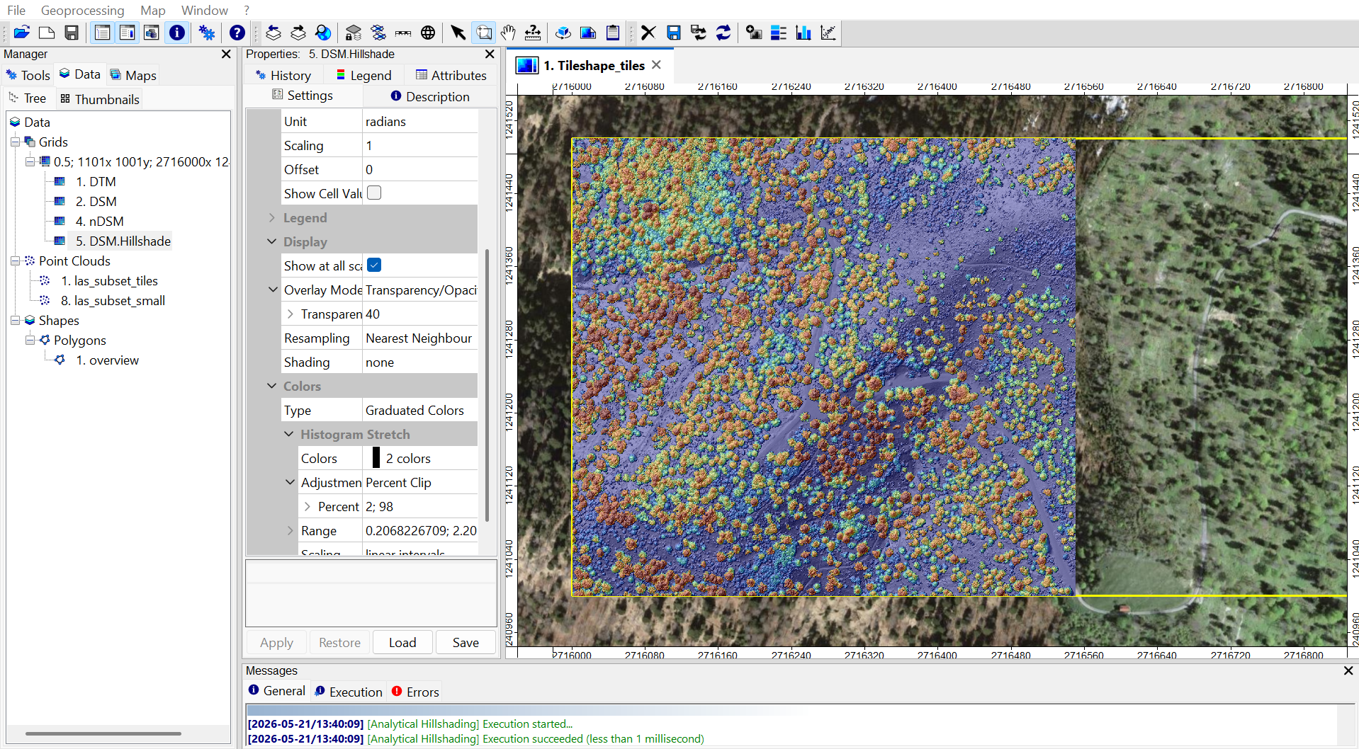
This will overlay the shading with the color-coding of the nDSM.
Save the Project (File > Project > Save Project) and close LIS Pro 3D.
Recap
In this tutorial section, we
- Queried a subset of the point cloud dataset
- Viewed the subset in the Point Cloud Editor
- Derived a
- Digital Surface Model (DSM)
- Digital Terrain Model (DTM)
- Normalized Digital Surface Model (nDSM)
- Created a Hillshade for visualization