Forestry Analysis
< Previous section Next section >
Recap
In the previous tutorial section, we
- Queried a subset of the point cloud dataset
- Viewed the subset in the Point Cloud Editor
- Derived a
- Digital Surface Model (DSM)
- Digital Terrain Model (DTM)
- Normalized Digital Surface Model (nDSM)
- Created a Hillshade for visualization
Start LIS Pro 3D
Search for LIS Pro 3D in your programs and start it!

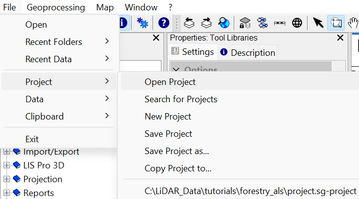
Open Project
Open the project from the previous tutorial section with all preprocessed datasets (e.g., DTM, DSM, nDSM, Hillshade)
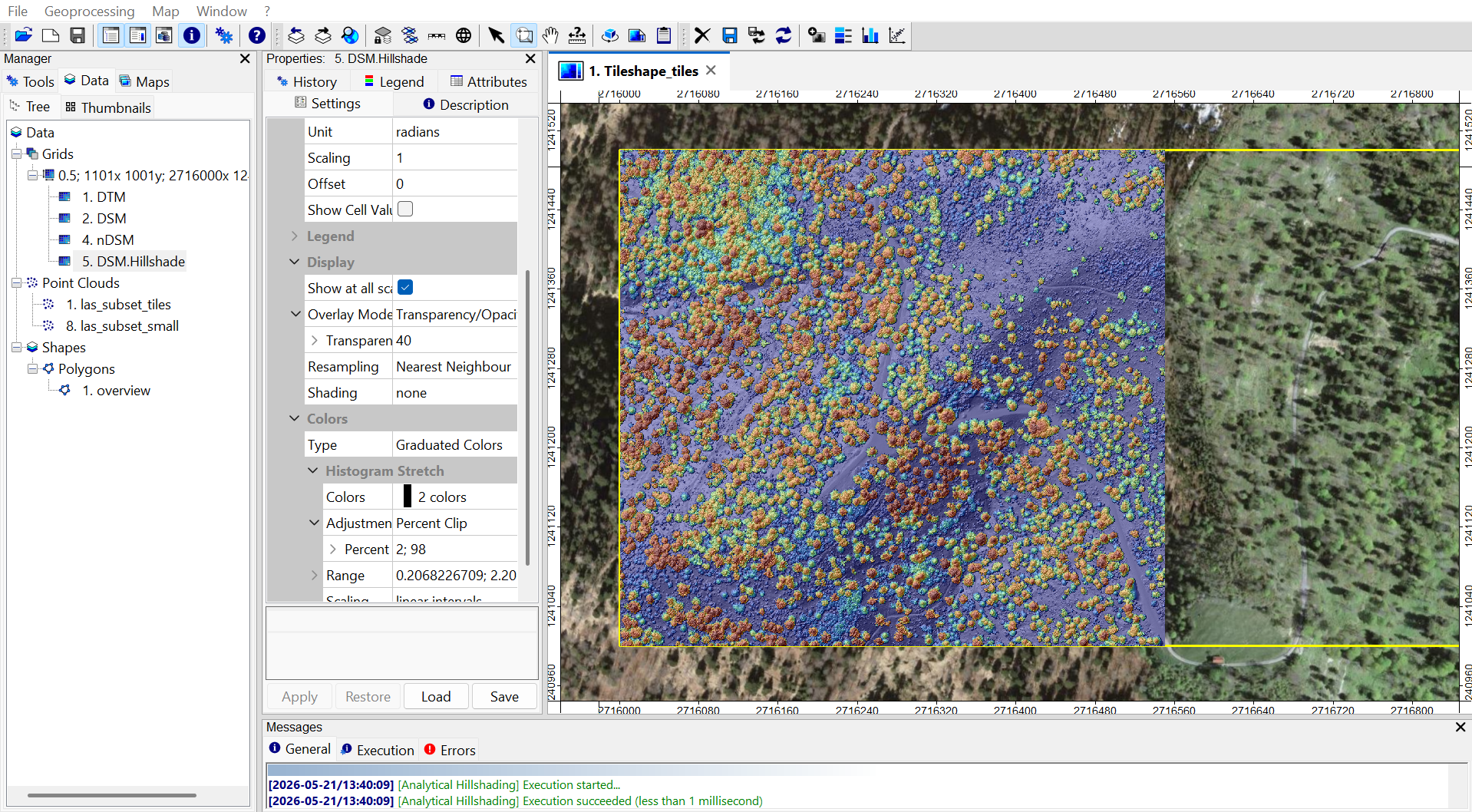
You should have the four grid datasets and at least the las_subset_tiles point cloud available from the previous tutorial section:
Generate High-Vegetation Mask
In this dataset low vegetation is defined as <3m, mid vegetation is defined as 3-10m and high vegetation is defined as >10m above ground.
A common dataset is a mask of the high vegetation. To create such a grid, use the Point Cloud to Grid tool and provide the following settings:
Tool: Point Cloud to Grid
Geoprocessing → LIS Pro 3D → Conversion → From Point Cloud // Tools → LIS Pro 3D → Conversion
| Parameter | Setting |
|---|---|
| Data Objects | |
| Point Clouds | |
| >> Point Cloud | las_subset_tiles |
| Attribute | classification |
| Filter Attribute | classification |
| Options | |
| Aggregation | max |
| Attribute Filter | ☐ |
| Elevation Filter | ☐ |
| Search Radius | ☐ |
| Filter Attribute Min / Max | 5;5 |
| Target Grid System | grid or grid system |
| Grid System | 0.5; 1001x, 1001y; 2716000…x 1241000…y |
| << Target Grid | <create> |
This will use the same grid system as the existing DEMs for the creation of the grid.
Click Execute.
This will create a new grid dataset, where all the valid grid cells have the value 5 (LAS classification id for high vegetation). The empty grid-cells are nodata. You can inspect the properties of the new layer by selecting it in the Data tab and looking into the Object Properties / Description tab.
In order to have a classical binary map available (with values 1 and nodata), reclassify the given grid, using the tool Reclassify Grid Values:
Tool: Reclassify Grid Values
Geoprocessing → Grid → Values // Tools → Grid → Tools
| Parameter | Setting |
|---|---|
| Data Objects | |
| Grids | |
| Grid System | 0.5; 1001x, 1001y; 2716000…x 1241000…y |
| >> Grid | Aggregate_classification_max |
| << Reclassified Grid | Reclassified Grid |
| Options | |
| Method | single |
| Old Value | 5 |
| New Value | 1 |
| Operator | = |
| Special Cases | |
| No Data Values | ☐ |
| Other Values | ☐ |
| Output Grid | |
| Data Storage Type | same as first grid in list |
| No Data Value | No Data value of input grid |
- Provide the available Grid System
- Provide the Aggregate_classification_max dataset in the Grid section
- Set the Old Value to 5
- Set the New Value to 1
- Click Execute
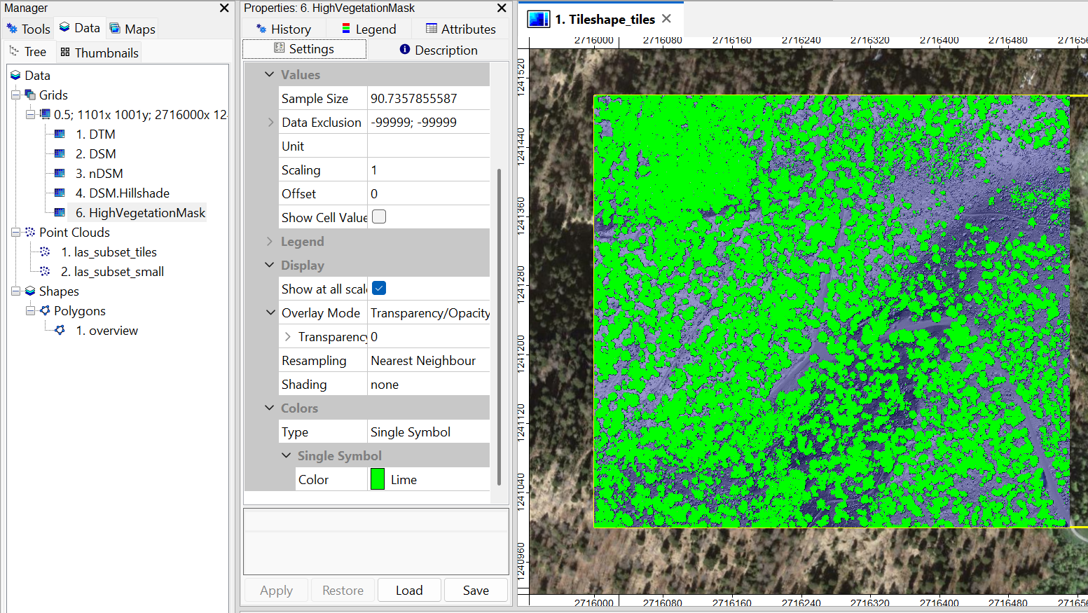
This creates a new dataset Aggregate_classification_max (Reclassified), which is our final high-vegetation-mask.
In the Settings of this new layer:
- Rename the layer to HighVegetationMask
- Set the Transparency to 40%
- Set the Colors > Type to Single Symbol
- Select Green as Color
- Click Apply
Additionally:
- Save the HighVegetationMask layer to disk
- Delete the temporary output layer Aggregate_classification_max
- Add the HighVegetationMask to the current map:
Attach DZ Value to Point Cloud
Similar to the generation of an nDSM, we want to add a new attribute to the table of the given point cloud. In the moment the point cloud imported from a laz-file has only the standard attributes available (e.g. intensity, classification), that can be inspected in the Description tab, if the point cloud is selected in the Data tab.
We have already a DTM available and can now add the height above ground (dz) to each individual laser point (using the given DTM)
Use the tool Height Above Ground from Grid and provide the following settings:
Tool: Height Above Ground from Grid
Geoprocessing → LIS Pro 3D → Arithmetic → Point Cloud // Tools → LIS Pro 3D → Arithmetic
| Parameter | Setting |
|---|---|
| Data Objects | |
| Grids | |
| Grid system | 0.5; 1001x, 1001y; 2716000…x 1241000…y |
| >> DEM | DTM |
| Point Clouds | |
| >> Point Cloud | las_subset_tiles |
| Copy existing attributes | 🗹 |
| < Point Cloud | <not set> |
| Attribute Suffix | |
| Options | |
| Method | vertical grid offset |
After execution, the point cloud has got a new attribute called dz.
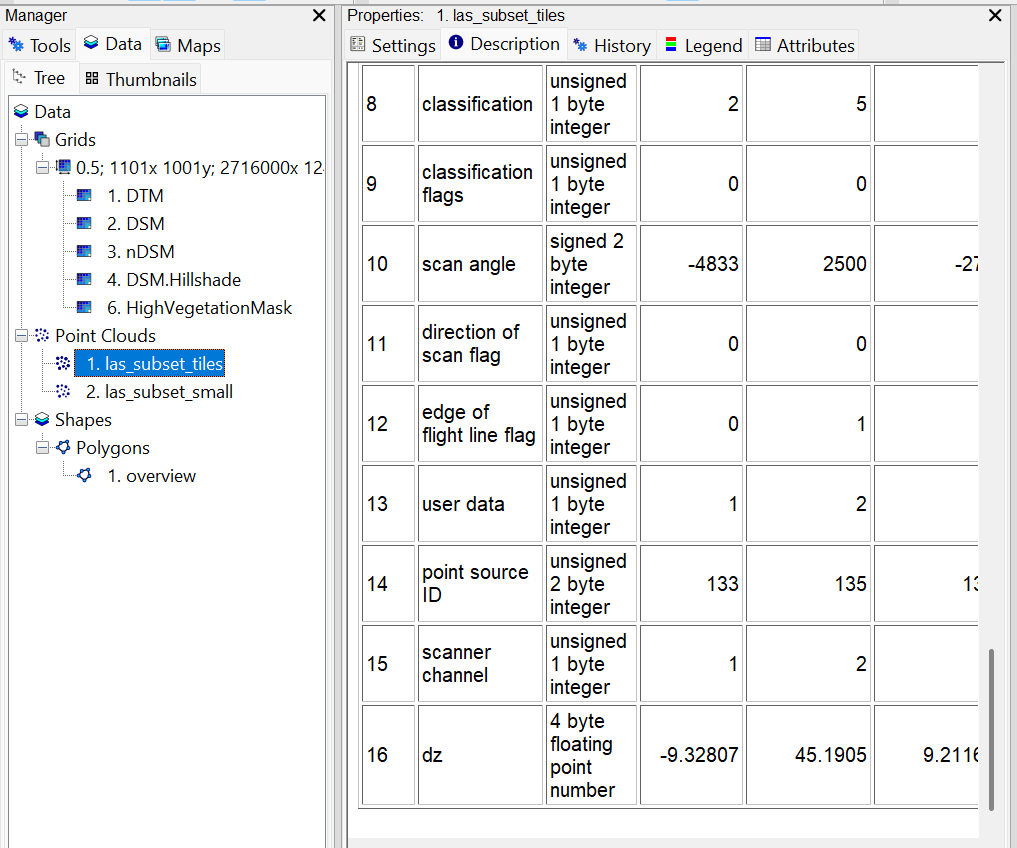
For the current dataset, the maximum tree height (indicated by the laser point with the maximum dz value) is around 45m.
Create Canopy Height Model
Create Canopy Height Model for the high-vegetation class (trees > 10m).
Again, use the tool Point Cloud to Grid with the following settings:
Tool: Point Cloud to Grid
Geoprocessing → LIS Pro 3D → Conversion → From Point Cloud // Tools → LIS Pro 3D → Conversion
| Parameter | Setting |
|---|---|
| Data Objects | |
| Point Clouds | |
| >> Point Cloud | las_subset_tiles |
| Attribute | dz |
| Filter Attribute | classification |
| Options | |
| Aggregation | max |
| Attribute Filter | ☐ |
| Elevation Filter | ☐ |
| Search Radius | ☐ |
| Filter Attribute Min / Max | 5;5 |
| Target Grid System | grid or grid system |
| Grid System | 0.5; 1001x, 1001y; 2716000…x 1241000…y |
| << Target Grid | <create> |
A new dataset has been created (Aggregate_dz_max). Rename it to CHM in Object Properties/Settings. Add the CHM to the map and hide all other datasets except the hillshade:
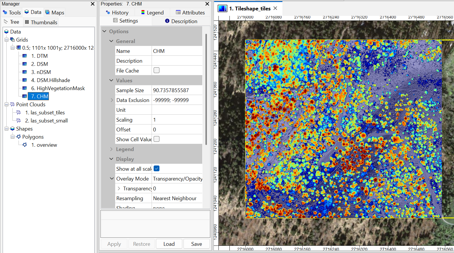
Save the CHM and the Project!
Smooth Canopy Height Model
Use the tool Gaussian Filter to smooth the canopy height model:
Tool: Gaussian Filter
Geoprocessing → Grid → Filter // Tools → Grid → Filter
| Parameter | Setting |
|---|---|
| Data Objects | |
| Grids | |
| Grid System | 0.5; 1101x, 1001y; 2716000…x 1241000…y |
| >> Grid | CHM |
| < Filtered Grid | |
| Options | |
| Kernel Radius | 4 |
| Standard Deviation | 50 |
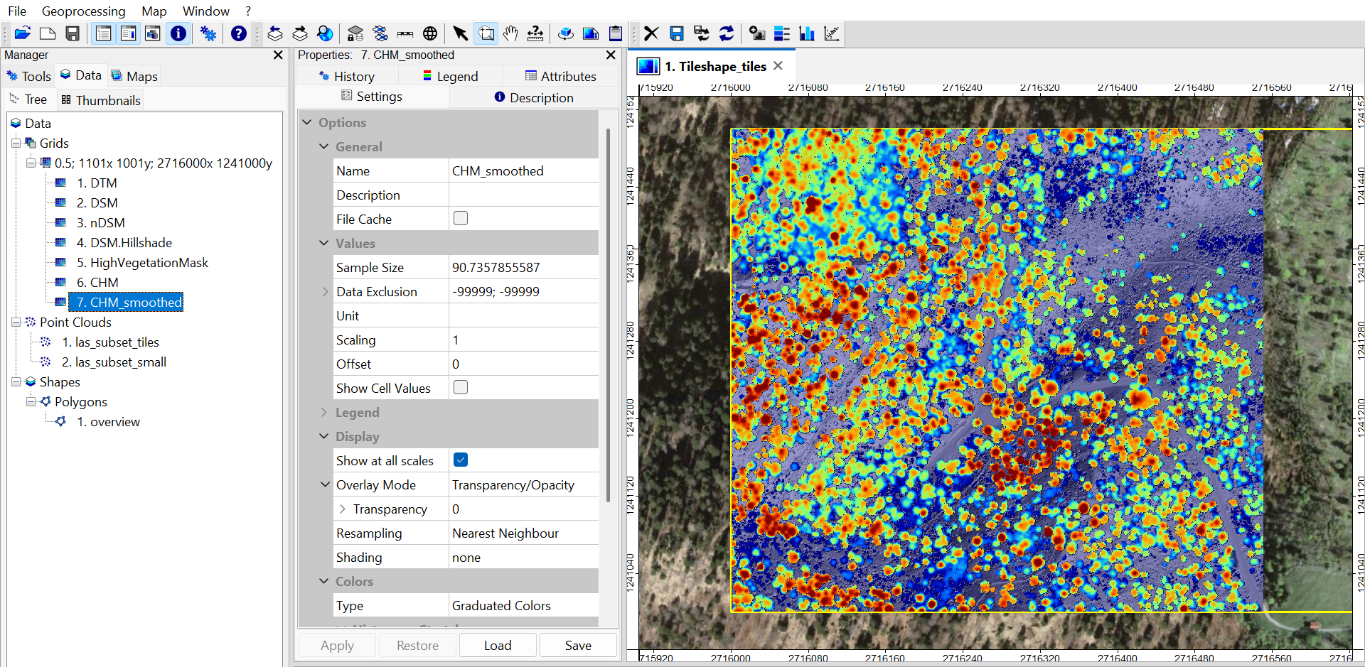
This will create a new dataset called CHM [Gaussian Filter]. Rename this dataset to CHM_smoothed.
Detect Single Trees
Use the tool Single Tree Detection in order to detect single trees:
Tool: Single Tree Derivation
Geoprocessing → LIS Pro 3D → Forestry → Grid // Tools → LIS Pro 3D → Forestry
| Parameter | Setting |
|---|---|
| Data Objects | |
| Grids | |
| Grid System | 0.5; 1001x, 1001y; 2716000…x 1241000…y |
| >> Canopy Height Model | CHM_smoothed |
| << Segments | <create> |
| Shapes | |
| << Seed Points | <create> |
| Options | |
| Allow Seeds on Grid Border | 🗹 |
| Segment Joining | seed to saddle difference |
| Threshold | 0.5 |
A new grid with tree segments (CHM_smoothed_segments) and a shapes layer with tree seeds (initial tree positions, CHM_smoothed_seeds ) have been generated. Set the Transparency of the CHM_smoothed_segments to 40% and add it to the map. Make all other datasets except for the hillshade invisible:
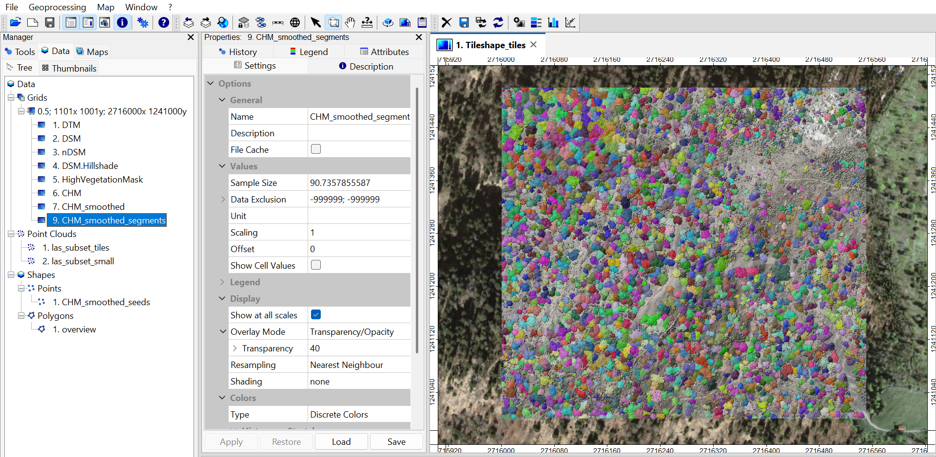
Save all datasets and save the project.
View Single Trees in 3D
Click onto the Show 3D-View button!
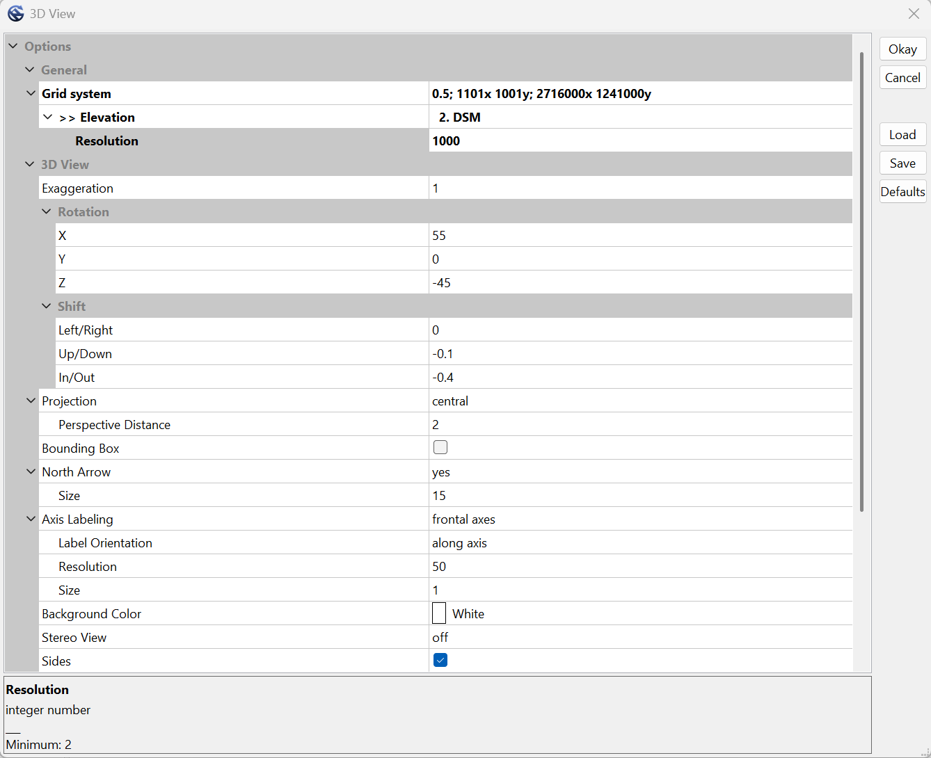
In the pop-up window:
- provide the available Grid System
- Provide the DSM dataset in the Elevation* section
- Set the Resolution to 1000
- Click Okay
A new tab opens in the maps panel. Now we can inspect the result of this segmentation in 3D:
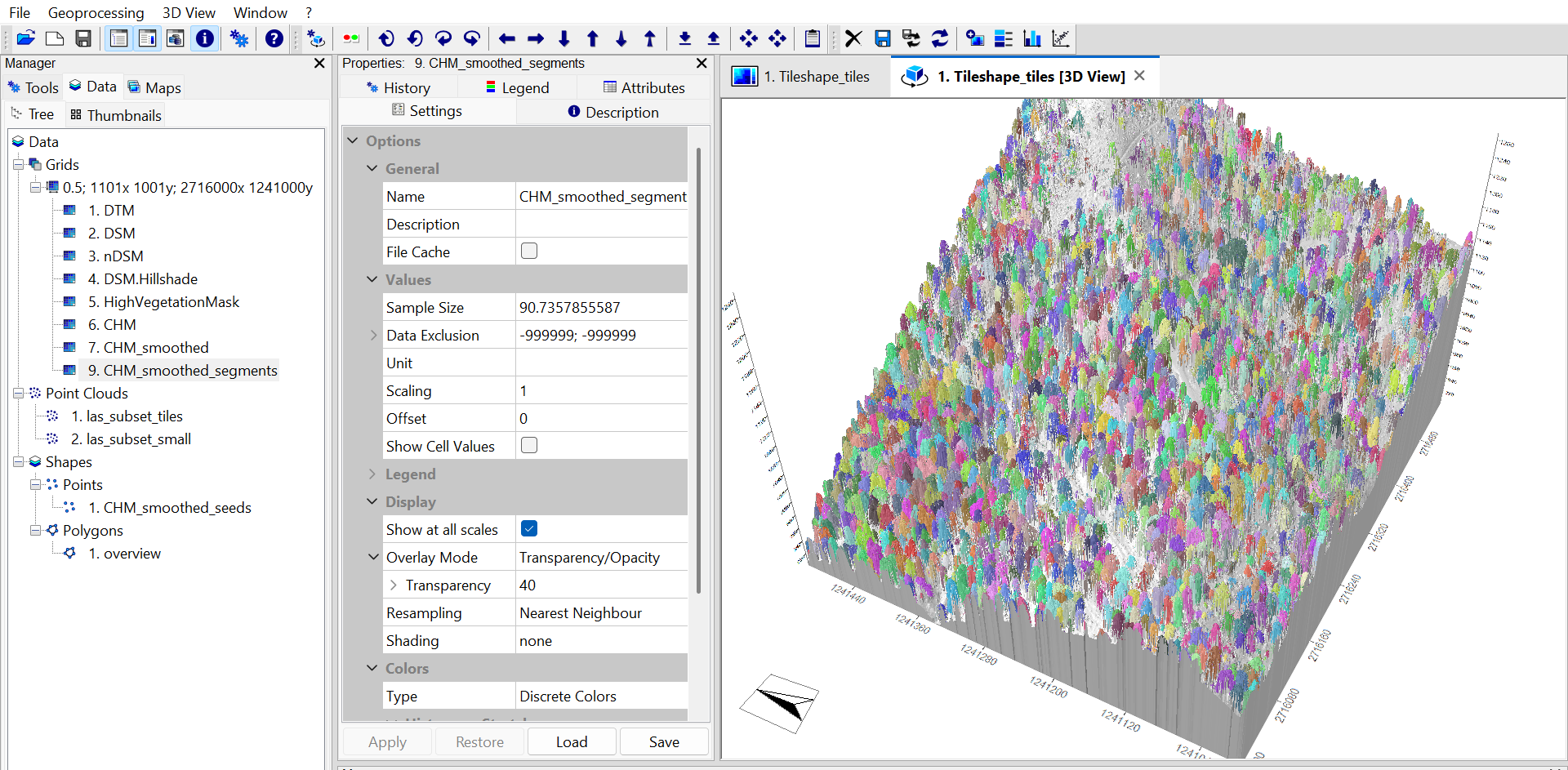
Close the 3D view tab again.
Rename the CHM_smoothed_segments to CHM_segments and the CHM_smoothed_seeds to CHM_seeds, in order to have shorter name.
Compute Single Tree Metrics
Use the tool Tree Shape Metrics in order to detect single trees:
Tool: Tree Shape Metrics
Geoprocessing → LIS Pro 3D → Forestry → Grid // Tools → LIS Pro 3D → Forestry
| Parameter | Setting |
|---|---|
| Data Objects | |
| Grids | |
| Grid System | 0.5; 1001x, 1001y; 2716000…x 1241000…y |
| >> Canopy Height Model | CHM |
| >> Crown Segments | CHM_segments |
| > DTM | <not set> |
| < Filtered Segments | <not set> |
| Shapes | |
| >> Seeds | CHM_seeds |
| << Treetops | <create> |
| < Centroids | <create> |
| < Boundaries | <create> |
| Smooth Boundaries | 🗹 |
| Options | |
| Apply Filter | 🗹 |
| Minimum Area | 2 |
| Minimum Shape Ratio | 0 |
| Create Trunk Positions | ☐ |
Note that we used a smoothed canopy height model for the segmentation, but used the original CHM for computing the metrics.
In the Data tab, two point layers have been added:
- CHM_segments_treetops (the tree top positions as shape layer)
- CHM_segments_centroids (the tree centroids as shape layer)
And one polygon layer has been added.
- CHM_segments_boundaries (the tree boundaries as shape layer)
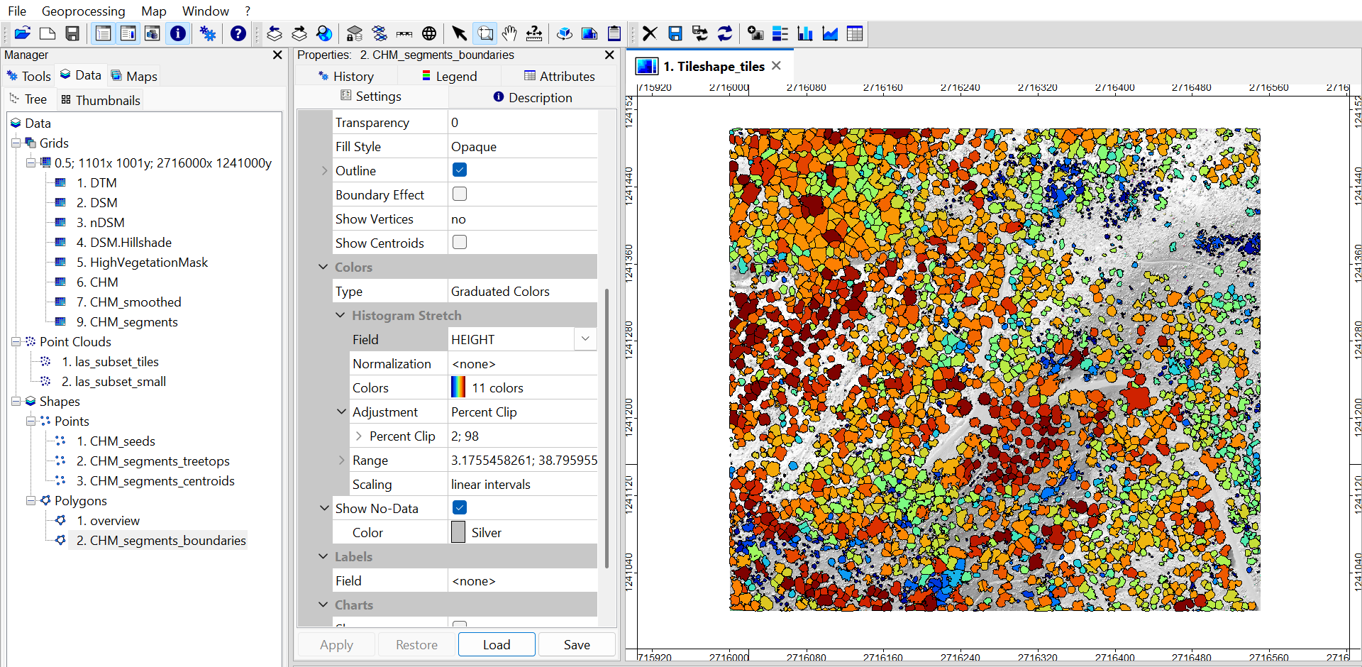
Add the CHM_segments_boundaries to the map!
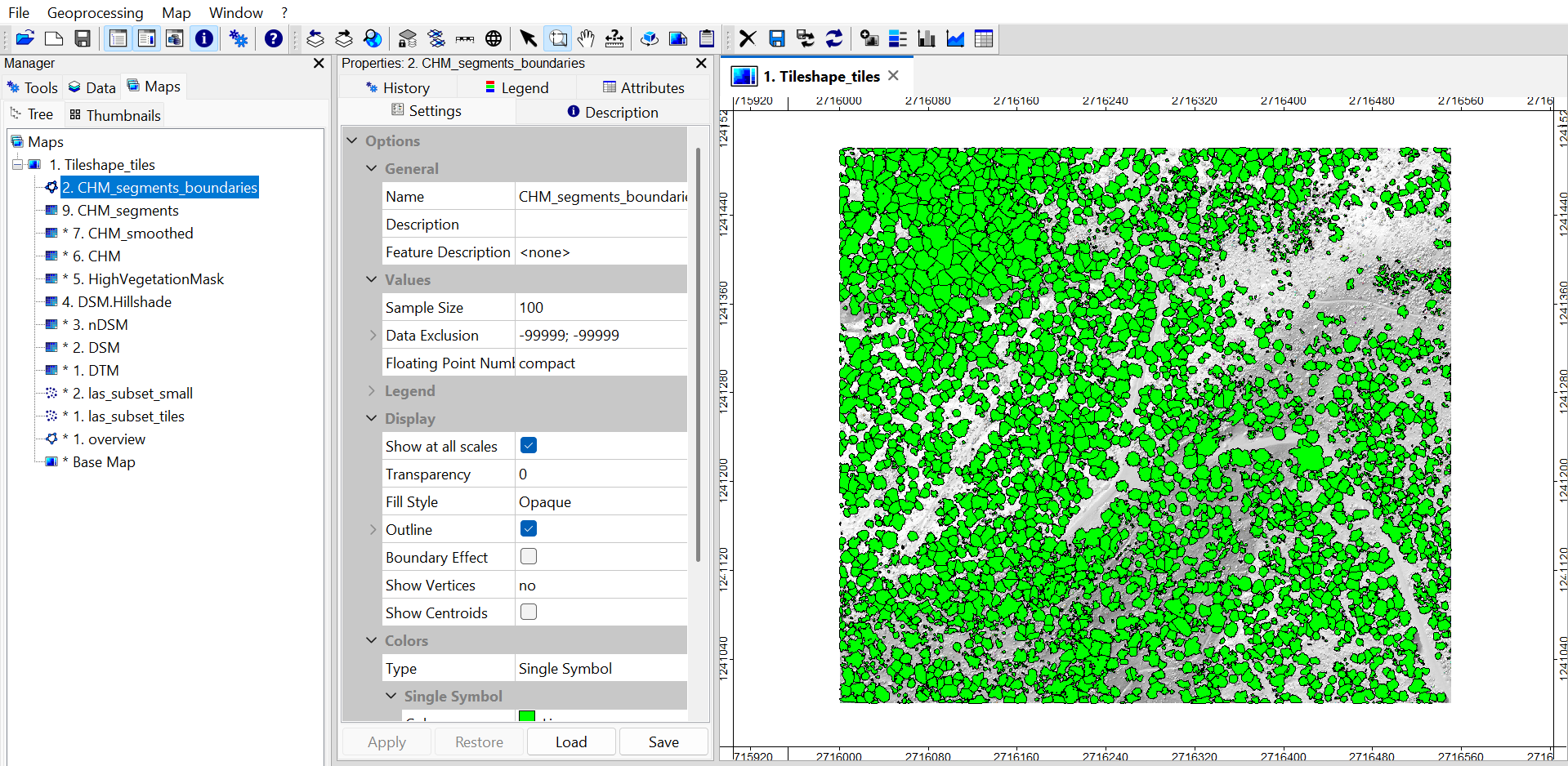
Each detected tree is now represented by a polygon.
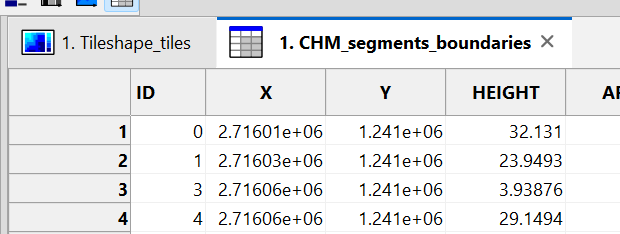
Right-click onto the boundaries layer in the Data tab in order to inspect its attribute table.
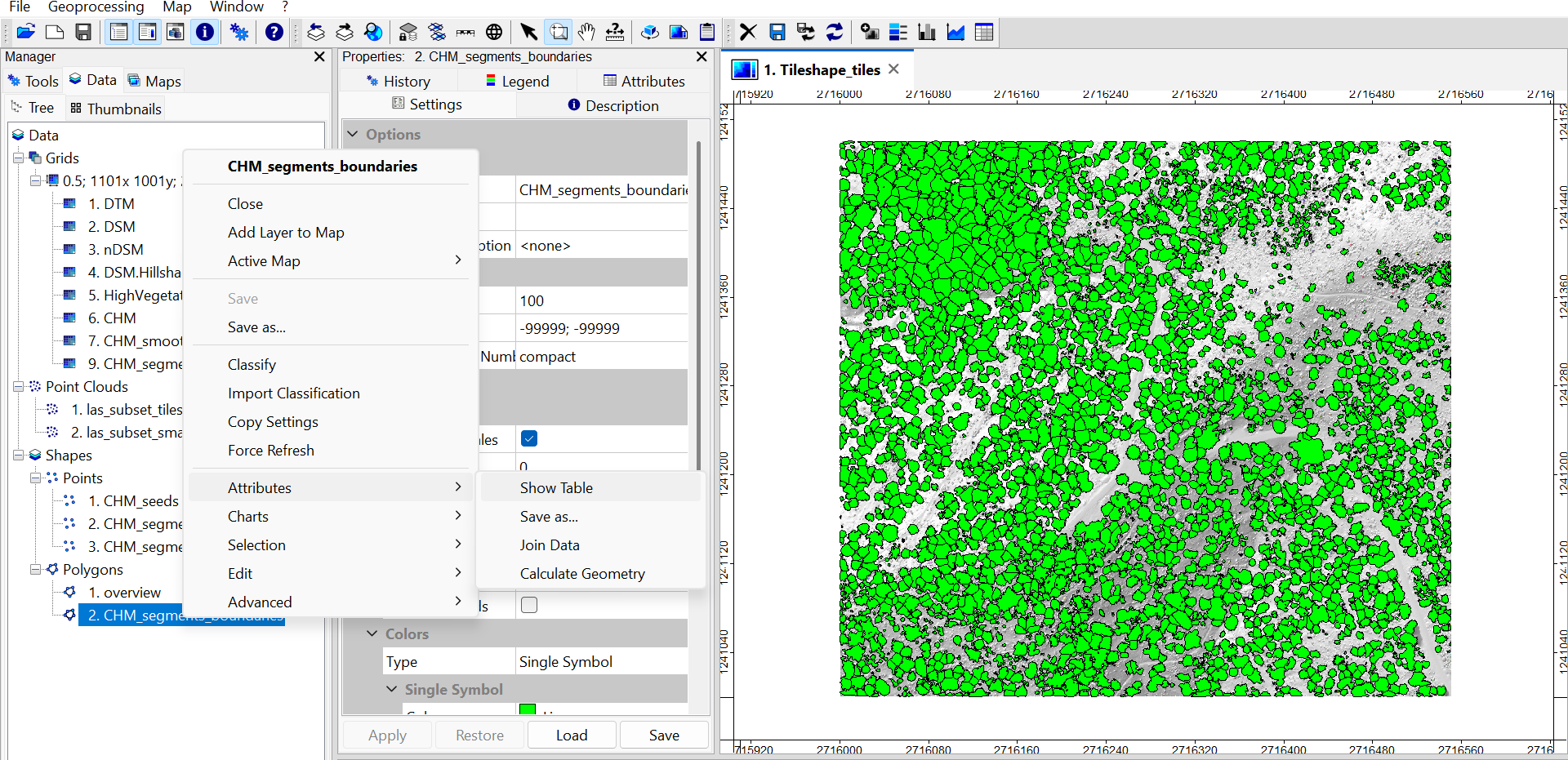
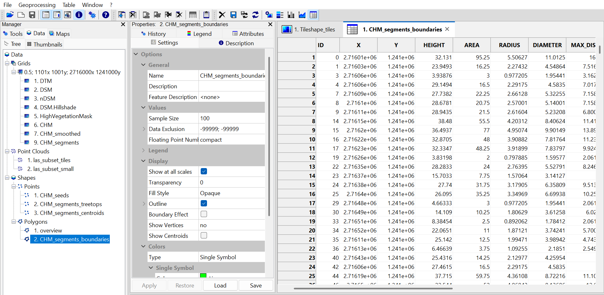
Each tree has one entry in the attributes table. Each tree has an xy-position, tree height (HEIGHT), crown area (AREA), crown radius and diameter (RADIUS & DIAMETER).
Close the table tab again!
Change Visualization of Boundaries
In the Settings of the boundaries layer
- set the Color > Type to Graduated Colors.
- set the Attribute to HEIGHT
Attach Segmentation to Point Cloud
Add the current segmentation to the input point cloud using the tool Attach Grid Values to Point Cloud:
Tool: Attach Grid Values to Point Cloud Geoprocessing → LIS Pro 3D → Tools → Point Cloud → Attributes // Tools → LIS Pro 3D → Tools
| Parameter | Setting |
|---|---|
| Data Objects | |
| Point Clouds | |
| >> Point Cloud | las_subset_tiles |
| Copy existing attributes | 🗹 |
| < Point Cloud | <not set> |
| Grids | |
| >> Grid(s) | 1 object (CHM_segments) |
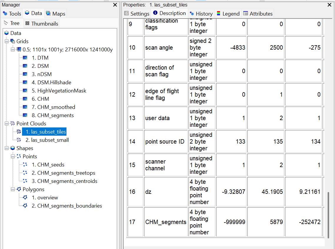
The point cloud has now an additional attribute called CHM_segments:
Clean Segmentation on Point Cloud
Right now, all points that fall into crown segments - including ground points - get a segment ID assigned . In order to improve the visualization, we will now relabel points < 0.5 m above ground and a segment ID < 1 (valid segment IDs start at 1) to the invalid class 0. Points above 0.5 m with a valid segment ID (>= 1) will retain their segment ID.
Tool: Attribute Filter
Geoprocessing → LIS Pro 3D → Filtering → Point Cloud // Tools → LIS Pro 3D → Filtering
| Parameter | Setting |
|---|---|
| Data Objects | |
| Point Clouds | |
| >> Point Cloud | las_subset_tiles |
| Attribute 1 | CHM_segments |
| Attribute 2 | dz |
| Attribute 3 | <not set> |
| Copy existing attributes | 🗹 |
| < Point Cloud | <not set> |
| Options | |
| Method | invalidate points |
| Attribute 1 | |
| Filter Type | lower limit (min) |
| Minimum | 1 |
| Attribute 2 | |
| Filter Type | lower limit (min) |
| Minimum | 0.5 |
| Attribute 3 | |
| Attribute Name | CHM_segments_clean |
| ID Invalid | 0 |
You may also choose to drop points below the thresholds in order to remove these points completely instead of invalidating them.
View Point Cloud Segmentation in 3D
Use the Point Cloud Editor to view the results:
Tool: Point Cloud Editor
Geoprocessing → LIS Pro 3D → Point Cloud Editor // Tools → LIS Pro 3D → Point Cloud Editor
| Parameter | Setting |
|---|---|
| Data Objects | |
| Point Clouds | |
| >> Point Cloud | las_subset_tiles |
| Intensity | intensity |
| RGB | <not set> |
| Shading | <not set> |
| Classification | <not set> |
| Random | CHM_segments_clean |
| Normal Vector (X) | <not set> |
| Report Attribute 1 | <not set> |
| Report Attribute 2 | <not set> |
| Grids | |
| > Elevation Grids | No objects |
| > Color Grids | No objects |
| Shapes | |
| > Shapes | <not set> |
| Options | |
| Work on Copy of Point Cloud | ☐ |
| Background Color | (60,60,50) |
In the Editor, type Q on the keyboard, in order to visualize the tree segments.
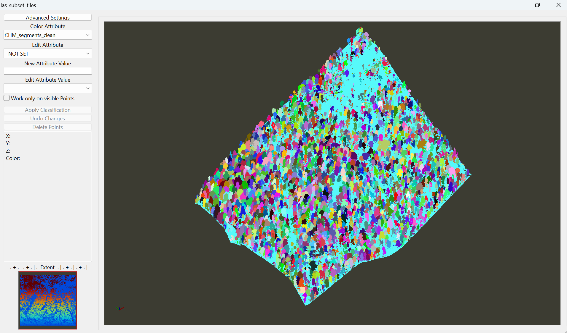
After you have inspected the point cloud, close the Editor again!
Save the project and close it!